Calculating Average Mountain Bike Speeds from GPX Tracks
In a discussion of ebikes on #BikeNite on Mastodon, someone mentioned speed limits she wouldn't mind being limited to, and that got me to wondering: how fast do I actually go on my bike?
I'm primarily a mountain biker. Most of my biking is either on dirt trails, or putting around town running errands. And my trail riding isn't super fast; I'm not one of those folks with the long-suspension bikes bombing down the ski runs at Pajarito. On the other hand, I do love a nice fast run on an up-and-down rollercoaster trail, and I really have no idea what sorts of top speeds I get to on these trails. But I track all my mountain bike rides with OsmAnd, so I have the data to figure it out.
As part of my PyTopo mapping program, I have a module called trackstats that can analyze a GPX file and find, among other things, maximum speed. So it was no problem to write a script that looks at all my mountain biking GPX files, finds the top speed from each, and then prints them all out along with an average.
Spikes
And the top speed was ... 49.66? That's obviously bogus. There's no way I'm ever going that fast on my mountain bike. Especially not on that track, "sherwood-muddy-2024-08-27.gpx" -- I'd noted in the filename that the track was muddy, so it was a fairly short run, I wasn't going my usual speeds and we were stopping a lot, and eventually we turned around because continuing would have left tracks in the trail.
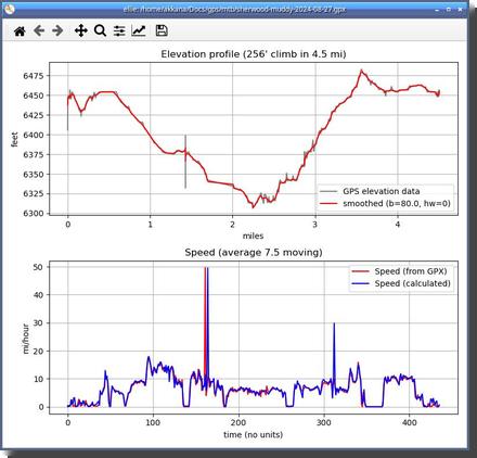 PyTopo has a companion program called Ellie that can plot speeds, both
speed in the GPX file and speed calculated from the GPX positions.
And the plot for that file was pretty interesting. Most of the speeds
were around 10-15, but there was one spike up to 30 plus the spike all the
way up to 50. This obviously wasn't real data, it was an artifact.
But that artifact was keeping me from knowing the real top speeds in my GPX files, so I had to solve it.
Interactive Plots
But first, I wanted more control over the plots. Ellie uses Python's matplotlib package. It's limited and frustrating to use: time axis labels are awful, and it's not interactive.
I recently added a "Show Charts for Track" option to PyTopo that gives an
interactive plot, so you can click on
a chart and see a marker on the map corresponding to that point in the chart.
But as yet it only plotted elevation and heart rate; I hadn't yet
added the capability to plot speeds. So I spent a few days adding plots
for speeds and other values,
and making sure the times on the X axis were properly labeled.
De-Spiking
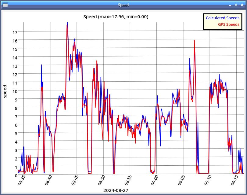
I already had a Kaiser window smoothing routine that I use for elevation, but I tried it on the speed data and to get rid of the spikes, I had to smooth the data too much, losing a lot of the real detail in the data.
I enlisted Claude's help, and got a nice Hampel despiking algorithm in numpy that got rid of the spikes without losing the rest of the detail.
Why the Spikes?
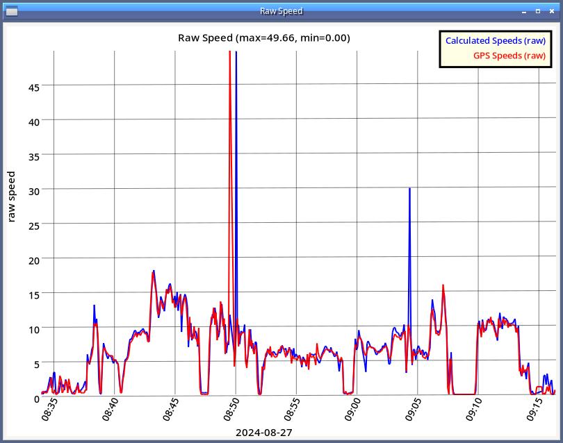
One interesting thing I noticed in the raw data was how the GPX speed (red) and the calculated speed (blue) both spiked to near 50, but not at exactly the same time. The calculated speed spiked a little later than the GPX. I might have written that off as an error in my plotting or data collection code — I'd had some other data alignment errors while debugging — but once I got those problems straightened out, the rest of the curves lined up so perfectly that I was pretty sure that the difference between the two spikes was real.
I located the section of the GPX where the spike happened, and uploaded that section to Claude, which gave me a great analysis:
The spike isn’t real, and the data shows why. It comes from a short burst of bad GPS fixes. What happened
time (UTC)	hdop	what the position did
14:50:09	4.5	good fix
(22 s with no points)
14:50:31	35	~113 m east of where you should be
14:50:36	35	still in the bad cluster
14:50:41	23.7	still in the bad cluster
14:50:46	7.1	snaps back onto the real track, ~110 m away in 5 s
HDOP is normally 4 to 5 for the rest of your file, so 35 means the receiver itself knew those fixes were junk. After the gap it reacquired with a badly displaced position, wandered around there for 10 seconds, then jumped back.
Why the two spikes are offset
GPX spike at 14:50:31: that’s the first bad fix, and the receiver reported 22.2 m/s (about 50 mph) for it. That’s probably the receiver reacting to its own position jump. The 22-second gap before it means a calculated speed over that segment is only about 5 m/s, so your calculation barely notices it.
Calculated spike at 14:50:46: the jump back to the good track covers about 110 m in 5 s, which is also about 22 m/s. Your calculation sees that jump. The receiver doesn’t flag it, because the new fix is good and its speed reads 4.3.
So both spikes come from the same glitch, one at each edge. The 14:50:46 time is 08:50:46 local (UTC-6), which matches your graph.
Claude also suggested that I drop points with a high hdop when calculating speed, perhaps with a threshold around 10. That sounds like a good idea that I'll probably pursue eventually.
Viewing the glitch
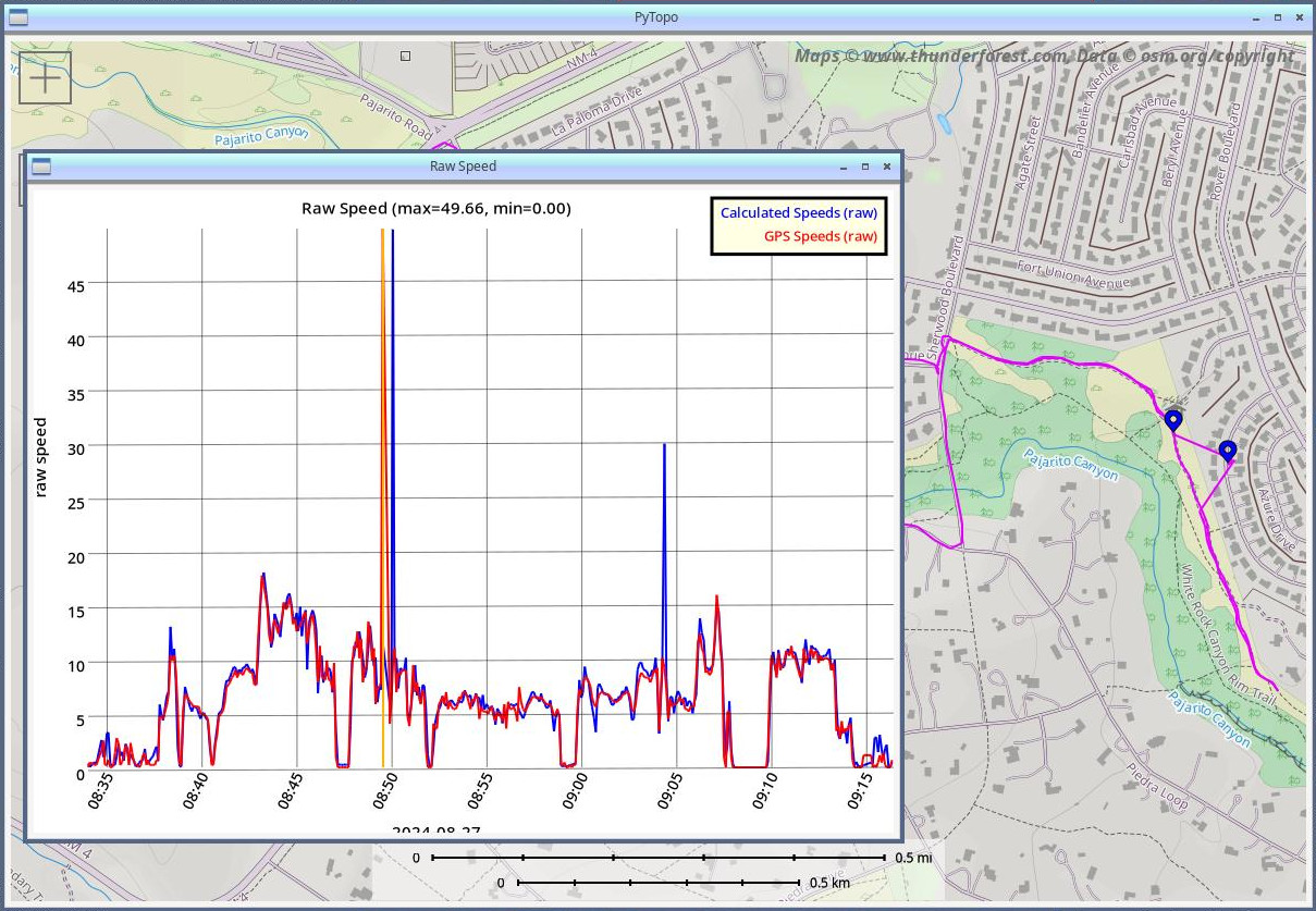 I mentioned earlier that my new plotting code lets you click on the
plot and see the corresponding point as markers on the map. I clicked on the
two spikes, and sure enough: you can see exactly where the GPX track
leaves the trail and wanders off into a neighborhood, and where it
goes back. So interesting!
What about those bike speed numbers?
What about the original question: how fast do I go on my mountain bike? Now that I had de-spiked data, I could answer that question. I went back to my original script and ran it on my collection of 261 GPX mountain biking track logs:
Highest speed: 20.35612033
Average max speed: 13.255852746248268

  0
  1
  2
  3 *
  4
  5
  6
  7 **
  8 **
  9 ******
 10 *******************
 11 ***********************************
 12 ***************************************************************
 13 *****************************************
 14 *****************************************************
 15 ***************
 16 ***********
 17 *****
 18 **
 19 ****
 20 *
(The number of stars is the number of rides on which my top speed was that speed, rounded down to the nearest integer. After all that work on the nice plots for PyTopo, ASCII graphics seemed good enough for this question.)
So I've never exceeded 21 mph on a trail, and on most of my rides, my highest speed is around 12 mph.
That's actually a little disappointing. I guess I'm not the speed demon I sometimes feel like I am when I'm bombing down the trail. But it's still good to have the numbers.
I added the script I used to find the top speeds to PyTopo: gpxspeeds.py in case other people might want to do a similar analysis.
[ 12:24 Nov 19, 2026 More mapping | permalink to this entry | ]


