I'm not sure where they got that idea; more science-leaning resources, like
Universe Today
and
Science Alert,
say 2024 is an "off" year for the Leonids,
with an expected Zenithal Hourly Rate (ZHR) of 15-20 meteors per hour
even with ideal conditions, which we don'e have because of an
almost-full moon.
The Tau Herculids come from periodic Comet 73P/Schwassmann-Wachmann, which
in 1995, began to break up, creating lots of debris scattered across
its orbit. It's hard to know exactly where the fragments ended up ...
but comet experts like Don Machholz think there's a good chance
that we'll be passing through an unusually dense clump of particles
when we cross 73P's orbit this year.
I'm not a big meteor watcher — I find most meteor showers
distinctly underwhelming. But in November 2001 (I think that's the right year),
I was lucky enough to view the Leonid meteor storm from
Fremont Peak, near San Juan Bautista, CA.
A couple of years ago, Dave and I acquired an H-alpha solar scope.
Neither of us had been much of a solar observer.
We'd only had white-light filters: filters you put over the
front of a regular telescope to block out most of the sun's light
so you can see sunspots.
H-alpha filters are a whole different beast:
you can see prominences, those huge arcs of fire that reach out into
space for tens of thousands of miles, many times the size of the Earth.
And you can also see all sorts of interesting flares and granulation
on the surface of the sun, something only barely hinted at in
white-light images.
I have another PEEC Planetarium talk coming up in a few weeks,
a talk on the
summer solstice
co-presenting with Chick Keller on Fri, Jun 18 at 7pm MDT.
I'm letting Chick do most of the talking about archaeoastronomy
since he knows a lot more about it than I do, while I'll be talking
about the celestial dynamics -- what is a solstice, what is the sun
doing in our sky and why would you care, and some weirdnesses relating
to sunrise and sunset times and the length of the day.
And of course I'll be talking about the analemma, because
just try to stop me talking about analemmas whenever the topic
of the sun's motion comes up.
But besides the analemma, I need a lot of graphics of the earth
showing the terminator, the dividing line between day and night.
Monday was the last night it's been clear enough to see Comet Neowise.
I shot some photos with the Rebel, but I haven't quite figured out
the alignment and stacking needed for decent astrophotos, so I don't
have much to show. I can't even see the ion tail.
The interesting thing about Monday besides just getting to see
the comet was the never-ending train of satellites.
Comet C/2020 F3 NEOWISE continues to improve, and as of Tuesday night
it has moved into the evening sky (while also still being visible in
the morning for a few more days).
I caught it Tuesday night at 9:30 pm. The sky was still a bit bright,
and although the comet was easy in binoculars, it was a struggle to see
it with the unaided eye. However, over the next fifteen minutes the sky
darkened, and it looked pretty good by 9:50, considering the partly
cloudy sky. I didn't attempt a photograph; this photo is from Sunday morning,
in twilight and with a bright moon.
I've learned not to get excited when I read about a new comet. They're
so often a disappointment. That goes double for comets in the morning
sky: I need a darned good reason to get up before dawn.
But the chatter among astronomers about the current comet, C2020 F3
NEOWISE, has been different. So when I found myself awake at 4 am,
I grabbed some binoculars and went out on the deck to look.
And I was glad I did. NEOWISE is by far the best comet I've seen
since Hale-Bopp. Which is not to say it's in Hale-Bopp's class --
certainly not. But it's easily visible to the unaided eye, with a
substantial several-degree-long tail. Even in dawn twilight. Even
with a bright moon. It's beautiful!
Update: the morning after I wrote that,
I did
get a photo,
though it's not nearly as good as Dbot3000's that's shown here.
Galen Gisler, our master of Planetarium Tricks,
presented something strange and cool in his planetarium show last Friday.
He'd been looking for a way to visualize
the "Venus Pentagram", a regularity where Venus'
inferior conjunctions -- the point where Venus is approximately
between Earth and the Sun -- follow a cycle of five.
If you plot the conjunction positions, you'll see a pentagram,
and the sixth conjunction will be almost (but not quite) in the
same place where the first one was.
Supposedly many ancient civilizations supposedly knew about this
pattern, though as Galen noted (and I'd also noticed when researching
my Stonehenge talk), the evidence is sometimes spotty.
Galen's latest trick: he moved the planetarium's observer location
up above the Earth's north ecliptic pole. Then he told the planetarium to
looked back at the Earth and lock the observer's position so it
moves along with the Earth; then he let the planets move in fast-forward,
leaving trails so their motions were plotted.
The result was fascinating to watch. You could see the Venus pentagram
easily as it made its five loops toward Earth, and the loops of all
the other planets as their distance from Earth changed over the course
of both Earth's orbits and theirs.
You can see the patterns they make at right, with the Venus pentagram
marked (click on the image for a larger version).
Venus' orbit is white, Mercury is yellow, Mars is red.
If you're wondering why Venus' orbit seems to go inside Mercury's,
remember: this is a geocentric model, so it's plotting distance from
Earth, and Venus gets both closer to and farther from Earth than Mercury does.
He said he'd shown this to the high school astronomy club and their
reaction was, "My, this is complicated." Indeed.
It gives insight into what a difficult problem geocentric astronomers
had in trying to model planetary motion, with their epicycles and
other corrections.
Of course that made me want one of my own. It's neat to watch it in
the planetarium, but you can't do that every day.
So: Python, Gtk/Cairo, and PyEphem. It's pretty simple, really.
The goal is to plot planet positions as viewed from high
above the north ecliptic pole: so for each time step, for each planet,
compute its right ascension and distance (declination doesn't matter)
and convert that to rectangular coordinates. Then draw a colored line
from the planet's last X, Y position to the new one. Save all the
coordinates in case the window needs to redraw.
At first I tried using Skyfield, the Python library which is supposed
to replace PyEphem (written by the same author). But Skyfield, while
it's probably more accurate, is much harder to use than PyEphem.
It uses SPICE kernels
(my blog post
on SPICE, some SPICE
examples and notes), which means there's no clear documentation or
list of which kernels cover what. I tried the kernels mentioned in the
Skyfield documentation, and after running for a while the program
died with an error saying its model for Jupiter in the de421.bsp kernel
wasn't good beyond 2471184.5 (October 9 2053).
Rather than spend half a day searching for other SPICE kernels,
I gave up on Skyfield and rewrote the program to use PyEphem,
which worked beautifully and amazed me with how much faster it was: I
had to rewrite my GTK code to use a timer just to slow it down to
where I could see the orbits as they developed!
It's fun to watch; maybe not quite as spacey as Galen's full-dome view
in the planetarium, but a lot more convenient.
You need Python 3, PyEphem and the usual GTK3 introspection modules;
on Debian-based systems I think the python3-gi-cairo package
will pull in most of them as dependencies.
I'm jazzed about this show. I think it'll be the most fun
planetarium show we've given so far.
We'll be showing a variety of lunarfeatures:
maria, craters, mountains, rilles, domes, catenae and more.
For each one, we'll discuss what the feature actually is and how it
was created, where to see good examples on the moon,
and -- the important part -- where you can go on Earth,
and specifically in the Western US,
to see a similar feature up close.
Plus: a short flyover of some of the major features using the
full-dome planetarium. Some features, like Tycho, the
Straight Wall, Reiner Gamma, plus lots of rilles, look really great
in the planetarium.
If you can't get to the moon yourself,
this is the next best thing!
The Hitchhiker's Guide to the Moon:
7pm at the PEEC nature center. Admission is free.
Come find out how to explore the moon without leaving your home planet!
The Mercury transit is over. But we learned some interesting things.
I'd seen Mercury transits before, but this is the first time we had an
H-alpha scope (a little 50mm Coronado PST) in addition to a white light
filter (I had my 102mm refractor set up with the Orion white-light filter).
As egress approached, Dave was viewing in the H-alpha while I was on
the white light scope. When I saw the black-drop effect at third
contact, Mercury was still nowhere near the edge in the H-alpha:
the H-alpha shows more of the solar atmosphere so the sun's image
is noticably bigger.
This was the point when we realized that we should have expected this
and been timing and recording. Alas, it was too late.
Mercury was roughly 60% out in the white light filter -- just past the
point where the "bite" it made in the limb of the sun -- by the time
Dave called out third contact. We guessed it was roughly a minute,
but that could be way off.
For fourth contact, Dave counted roughly 45 seconds between when I
couldn't see Mercury any more and when he lost track of it. This is
pretty rough, because it was windy, seeing was terrible and there
was at least a 15-second slop when I wasn't sure if I could any
indentation in the limb; I'm sure it was at least as hard in the
Coronado, which was running at much lower magnification.
So we had a chance to do interesting science and we flubbed it.
And the next chance isn't til 2032; who knows if we'll still be
actively observing then.
I wanted to at least correlate those two numbers: 45 seconds and
60% of a Mercury radius.
Mercury is about 10" (arcseconds) right now. That was easy to find.
But how fast does it move? I couldn't find anything about that,
searching for terms like mercury transit angular speed OR velocity.
I tried to calculate it with PyEphem but got a number that was orders of
magnitude off. Maybe I'll figure it out for a later article, but I wanted
to get this posted quickly.
I didn't spend much time trying photography. I got a couple afocal snaps with
my pocket digital camera through the white-light scope that worked out pretty well.
I wasn't sure that would work for the Coronado: the image is fairly dim.
The snaps I did get show Mercury, though none of the interesting detail
like faculae and the one tiny prominence that was visible. But the
interesting thing is the color. To the eye, the H-alpha scope image is
a slightly orangy red, but in the digital camera it came out a
startling purplish pink. This may be due to the digital camera's filters
passing some IR, confusing the algorithms that decide how to shift the color.
Of course, I could have adjusted the color in GIMP back to the real color,
but I thought it was more interesting to leave it the hue it came out
of the camera. (I did boost contrast and run an unsharp mask filter, to
make it easier to see Mercury.)
Anyway, fun and unexpectedly edifying! I wish we had another transit
happening sooner than 2032.
Mercury Transit 2006, photo by Brocken Inaglory
Next Monday, November 11, is a transit of Mercury across the sun.
Mercury transits aren't super rare -- not once- or twice-in-a-lifetime
events like
Venus
transits -- but they're not that common, either.
The last Mercury transit was in 2016; the next one won't happen til 2032.
This year's transit isn't ideal for US observers. The transit will
already be well underway by the time the sun rises, at least in the
western US. Here in New Mexico (Mountain time), the sun rises with
Mercury transiting, and the transit lasts until 11:04 MST.
Everybody else, check
timeanddate's
Mercury Transit page for your local times.
Mercury is small, unfortunately, so it's not an easy thing to see
without magnification. Of course, you know that
you should never look at the sun without an adequate filter.
But even if you have safe "eclipse glasses", it may be tough to
spot Mercury's small disk against the surface of the sun.
One option is to take some binoculars and use them to project an image.
Point the big end of the binoculars at the sun, and the small end at
a white surface, preferably leaning so it's perpendicular to the sun.
I don't know if binocular projection will give a big enough image
to show Mercury, so a very smooth and white background, tilted so
it's perpendicular to the sun, will help.
(Don't be tempted to stick eclipse glasses in front of a
binocular or telescope and look through the eyepiece! Stick to
projection unless you have filters specifically intended for
telescopes or binoculars.)
Of course, a telescope with a safe solar filter is the best way to see a
transit. If you're in the Los Alamos area, I hear the Pajarito
Astronomers are planning to set up telescopes at Overlook Park.
They don't seem to have announced it in any of the papers yet, but
I see it listed on the
Pajarito Astronomers
website.
There's also an event planned at the high school where the students
will be trying to time Mercury's passage, but I don't know if
that's open to the public. Elsewhere in the world, check with your local
astronomy club for Mercury transit parties: I'm sure most clubs have
something planned.
I was discussing the transit with a couple of local astronomers earlier
this week, and one of them related it to the search for exoplanets.
One of the main methods of detecting exoplanets is to measure the dimming
of a star's light as a planet crosses its face.
For instance, in
55 Cancri e,
you can see a dimming as the planet crosses the star's face, and a
much more subtle dimming when the planet disappears behind the star.
As Mercury crosses the Sun's face, it blocks some of the sun's light
in the same way. By how much?
The radius of Mercury is 0.0035068 solar radii, and the dimming is
proportional to area so it should be 0.00350682, or
0.0000123, a 0.00123% dimming. Not very much!
But it looks like in the 55 Cancri e case, they're detecting dips
of around .001% -- it seems amazing that you could detect a planet
as small as Mercury this way (and certainly the planet is much bigger
in the case of 55 Cancri e) ... but maybe it's possible.
Anyway, it's fun to think about exoplanets as you watch tiny Mercury
make its way across the face of the Sun.
Wherever you are, I hope you get a chance to look!
For those who haven't already read about the issue in the national
press, New Mexico's Public Education Department (a body appointed by
the governor) has a proposal regarding new science standards for all
state schools. The proposal starts with the national
Next Generation Science Standards
but then makes modifications, omitting points like references to
evolution and embryological development or the age of the Earth
and adding a slew of NM-specific standards that are mostly
sociological rather than scientific.
New Mexico residents have until 5.p.m. next Monday, October 16, to speak
out about the proposal.
Email comments to
rule.feedback@state.nm.us
or send snail mail (it must arrive by Monday) to
Jamie Gonzales, Policy Division, New Mexico Public Education Department,
Room 101, 300 Don Gaspar Avenue, Santa Fe, New Mexico 87501.
A few excellent letters people have already written:
I'm sure they said it better than I can. But every voice counts --
they'll be counting letters! So here's my letter. If you live in New
Mexico, please send your own. It doesn't have to be long: the
important thing is that you begin by stating your position on
the proposed standards.
Members of the PED:
Please reconsider the proposed New Mexico STEM-Ready Science Standards,
and instead, adopt the nationwide Next Generation Science Standards
(NGSS) for New Mexico.
With New Mexico schools ranking at the bottom in every national
education comparison, and with New Mexico hurting for jobs and having
trouble attracting technology companies to our state, we need our
students learning rigorous, established science.
The NGSS represents the work of people in 26 states, and
is being used without change in 18 states already. It's been well
vetted, and there are many lesson plans, textbooks, tests and other
educational materials available for it.
The New Mexico Legislature supports NGSS: they passed House Bill 211
in 2017 (vetoed by Governor Martinez) requiring adoption of the NGSS.
The PED's own Math and Science Advisory Council (MSAC) supports NGSS:
they recommended in 2015 that it be adopted. Why has the PED ignored
the legislature and its own advisory council?
Using the NGSS without New Mexico changes will save New Mexico money.
The NGSS is freely available. Open source textbooks and lesson plans
are already available for the NGSS, and more are coming. In contrast,
the New Mexico Stem-Ready standards would be unique to New Mexico:
not only would we be left out of free nationwide educational materials,
but we'd have to pay to develop New Mexico-specific curricula and
textbooks that couldn't be used anywhere else, and the resulting
textbooks would cost far more than standard texts. Most of this money
would go to publishers in other states.
New Mexico consistently ranks at the bottom in educational
comparisons. Yet nearly 15% of the PED's proposed stem-ready standards
are New Mexico specific standards, taught nowhere else, and will take
time away from teaching core science concepts. Where is the evidence
that our state standards would be better than what is taught in other
states? Who are we to think we can write better standards than a
nationwide coalition?
In addition, some of the changes in the proposed NM STEM-Ready Science
Standards seem to be motivated by political ideology, not science.
Science standards used in our schools should be based on widely
accepted scientific principles. Not to mention that the national
coverage on this issue is making our state a laughingstock.
Finally, the lack of transparency in the NMSRSS proposal is alarming.
Who came up with the proposed NMSRSS standards? Are there any experts
in science education that support them? Is there any data to indicate
they'd be more effective than the NGSS? Why wasn't the development of
the NMSRSS discussed in open PED meetings as required by the Open
Meetings Act?
The NGSS are an established, well regarded national standard. Don't
shortchange New Mexico students by teaching them watered-down science.
Please discard the New Mexico Stem-Ready proposal and adopt the Next
Generation Science Standards, without New Mexico-specific changes.
Late notice, but Dave and I are giving a talk on the moon
tonight at PEEC. It's called
Moonlight
Sonata, and starts at 7pm. Admission: $6/adult, $4/child
(we both prefer giving free talks, but PEEC likes to charge for
their Friday planetarium shows, and it all goes to support PEEC,
a good cause).
We'll bring a small telescope in case anyone wants to do any actual
lunar observing outside afterward, though usually planetarium
audiences don't seem very interested in that.
If you're local but can't make it this time, don't worry; the moon
isn't a one-time event, so I'm sure we'll give the moon show again at
some point.
I haven't had a chance to do much astronomy since moving to New Mexico,
despite the stunning dark skies. For one thing, those stunning dark
skies are often covered with clouds -- New Mexico's dramatic skyscapes
can go from clear to windy to cloudy to hail or thunderstorms and back
to clear and hot over the course of a few hours. Gorgeous to watch,
but distracting for astronomy, and particularly bad if you want to
plan ahead and observe on a particular night. The Pajarito Astronomers'
monthly star parties are often clouded or rained out, as was the PEEC
Nature Center's moon-and-planets star party last week.
That sort of uncertainty means that the best bet is a so-called
"quick-look scope": one that sits by the door, ready to be hauled
out if the sky is clear and you have the urge.
Usually that means some kind of tiny refractor; but it can also
mean leaving a heavy mount permanently set up (with a cover to protect
it from those thunderstorms) so it's easy to carry out a telescope
tube and plunk it on the mount.
I have just that sort of scope sitting in our shed: an old, dusty Cave
Astrola 6" Newtonian on an equatorian mount.
My father got it for me on my 12th birthday.
Where he got the money for such a princely gift -- we didn't have
much in those days -- I never knew, but I cherished that telescope,
and for years spent most of my nights in the backyard peering through
the Los Angeles smog.
Eventually I hooked up with older astronomers (alas, my father had
passed away) and cadged rides to star parties out in the Mojave desert.
Fortunately for me, parenting standards back then allowed a lot
more freedom, and my mother was a good judge of character and let
me go. I wonder if there are any parents today who would let their
daughter go off to the desert with a bunch of strange men? Even back
then, she told me later, some of her friends ribbed her -- "Oh,
'astronomy'. Suuuuuure. They're probably all off doing drugs in the desert."
I'm so lucky that my mom trusted me (and her own sense of the guys
in the local astronomy club) more than her friends.
The Cave has followed me through quite a few moves, heavy, bulky and
old fashioned as it is; even when I had scopes
that were bigger, or more portable, I kept it for the sentimental value.
But I hadn't actually set it up in years. Last week, I assembled the
heavy mount and set it up on a clear spot in the yard. I dusted off
the scope, cleaned the primary mirror and collimated everything,
replaced the finder which had fallen out somewhere along the way,
set it up ... and waited for a break in the clouds.
I'm happy to say that the optics are still excellent.
As I write this (to be posted later),
I just came in from beautiful views of Hyginus Rille and the
Alpine Valley on the moon. On Jupiter the Great Red Spot was just
rotating out. Mars, a couple of weeks before opposition, is still
behind a cloud (yes, there are plenty of clouds). And now the clouds
have covered the moon and Jupiter as well. Meanwhile, while I wait for
a clear view of Mars, a bat makes frenetic passes overhead, and
something in the junipers next to my observing spot is making rhythmic
crunch, crunch, crunch sounds. A rabbit chewing something tough?
Or just something rustling in the bushes?
I just went out again,
and now the clouds have briefly uncovered Mars. It's the first good look
I've had at the Red Planet in years. (Tiny achromatic refractors really
don't do justice to tiny, bright objects.) Mars is the most difficult
planet to observe: Dave liks to talk about needing to get your "Mars
eyes" trained for each Mars opposition, since they only come every two
years. But even without my "Mars eyes", I had no trouble seeing the
North pole with dark Acidalia enveloping it, and, in the south, the
sinuous chain of Sini Sabaeus, Meridiani, Margaritifer, and Mare Erythraeum.
(I didn't identify any of these at the time; instead, I dusted off my
sketch pad and sketched what I saw, then compared it with XEphem's
Mars view afterward.)
I'm liking this new quick-look telescope -- not to mention the
childhood memories it brings back.
We had perfect weather for the partial solar eclipse yesterday.
I invited some friends over for an eclipse party -- we set up
a couple of scopes with solar filters, put out food and drink
and had an enjoyable afternoon.
And what views! The sunspot group right on the center of the sun's disk
was the most large and complex I'd ever seen, and there were some much
smaller, more subtle spots in the path of the eclipse. Meanwhile, the
moon's limb gave us a nice show of mountains and crater rims silhouetted
against the sun.
I didn't do much photography, but I did hold the point-and-shoot up to
the eyepiece for a few shots about twenty minutes before maximum eclipse,
and was quite pleased with the result.
An excellent afternoon. And I made too much blueberry bread and
far too many oatmeal cookies ... so I'll have sweet eclipse memories
for quite some time.
Finding separation between two objects is easy in PyEphem: it's just one
line once you've set up your objects, observer and date.
p1 = ephem.Mars()
p2 = ephem.Jupiter()
observer = ephem.Observer()  # and then set it to your city, etc.
observer.date = ephem.date('2014/8/1')
p1.compute(observer)
p2.compute(observer)

ephem.separation(p1, p2)
So all I have to do is loop over all the visible planets and see when
the separation is less than some set minimum, like 4 degrees, right?
Well, not really. That tells me if there's a conjunction between
a particular pair of planets, like Mars and Jupiter. But the really
interesting events are when you have three or more objects close
together in the sky. And events like that often span several days.
If there's a conjunction of Mars, Venus, and the moon, I don't want to
print something awful like
Friday:
  Conjunction between Mars and Venus, separation 2.7 degrees.
  Conjunction between the moon and Mars, separation 3.8 degrees.
Saturday:
  Conjunction between Mars and Venus, separation 2.2 degrees.
  Conjunction between Venus and the moon, separation 3.9 degrees.
  Conjunction between the moon and Mars, separation 3.2 degrees.
Sunday:
  Conjunction between Venus and the moon, separation 4.0 degrees.
  Conjunction between the moon and Mars, separation 2.5 degrees.
... and so on, for each day. I'd prefer something like:
Conjunction between Mars, Venus and the moon lasts from Friday through Sunday.
  Mars and Venus are closest on Saturday (2.2 degrees).
  The moon and Mars are closest on Sunday (2.5 degrees).
At first I tried just keeping a list of planets involved in the conjunction.
So if I see Mars and Jupiter close together, I'd make a list [mars,
jupiter], and then if I see Venus and Mars on the same date, I search
through all the current conjunction lists and see if either Venus or
Mars is already in a list, and if so, add the other one. But that got
out of hand quickly. What if my conjunction list looks like
[ [mars, venus], [jupiter, saturn] ] and then I see there's also
a conjunction between Mars and Jupiter? Oops -- how do you merge
those two lists together?
The solution to taking all these pairs and turning them into a list
of groups that are all connected actually lies in graph theory: each
conjunction pair, like [mars, venus], is an edge, and the trick is to
find all the connected edges. But turning my list of conjunction pairs
into a graph so I could use a pre-made graph theory algorithm looked
like it was going to be more code -- and a lot harder to read and less
maintainable -- than making a bunch of custom Python classes.
I eventually ended up with three classes:
ConjunctionPair, for a single conjunction observed between two bodies
on a single date;
Conjunction, a collection of ConjunctionPairs covering as many bodies
and dates as needed;
and ConjunctionList, the list of all Conjunctions currently active.
That let me write methods to handle merging multiple conjunction
events together if they turned out to be connected, as well as a
method to summarize the event in a nice, readable way.
So predicting conjunctions ended up being a lot more code than I
expected -- but only because of the problem of presenting it neatly
to the user. As always, user interface represents the hardest part
of coding.
All through the years I was writing the planet observing column for
the San Jose Astronomical Association, I was annoyed at the lack of places
to go to find out about upcoming events like conjunctions, when two or
more planets are close together in the sky. It's easy to find out
about conjunctions in the next month, but not so easy to find sites
that will tell you several months in advance, like you need if you're
writing for a print publication (even a club newsletter).
For some reason I never thought about trying to calculate it myself.
I just assumed it would be hard, and wanted a source that could
spoon-feed me the predictions.
The best source I know of is the
RASC Observer's Handbook,
which I faithfully bought every year and checked each month so I could
enter that month's events by hand. Except for January and February, when I
didn't have the next year's handbook yet by the time my column went
to press and I was on my own.
I have to confess, I was happy to get away from that aspect of the
column when I moved.
In my new town, I've been helping the local nature center with their
website. They had some great pages already, like a
What's
Blooming Now? page that keeps track
of which flowers are blooming now and only shows the current ones.
I've been helping them extend it by adding features like showing only
flowers of a particular color, separating the data into CSV databases
so it's easier to add new flowers or butterflies, and so forth.
Eventually we hope to build similar databases of birds, reptiles and
amphibians.
And recently someone suggested that their astronomy page could use
some help. Indeed it could -- it hadn't been updated in about five years.
So we got to work looking for a source of upcoming astronomy events
we could use as a data source for the page, and we found sources for
a few things, like moon phases and eclipses, but not much.
Someone asked about planetary conjunctions, and remembering
how I'd always struggled to find that data, especially in months when
I didn't have the RASC handbook yet, I got to wondering about
calculating it myself.
Obviously it's possible to calculate when a planet will
be visible, or whether two planets are close to each other in the sky.
And I've done some programming with
PyEphem before, and found
it fairly easy to use. How hard could it be?
Note: this article covers only the basic problem of predicting when
a planet will be visible in the evening.
A followup article will discuss the harder problem of conjunctions.
Calculating planet visibility with PyEphem
The first step was figuring out when planets were up.
That was straightforward. Make a list of the easily visible planets
(remember, this is for a nature center, so people using the page
aren't expected to have telescopes):
Then we need an observer with the right latitude, longitude and
elevation. Elevation is apparently in meters, though they never bother
to mention that in the PyEphem documentation:
observer = ephem.Observer()
observer.name = "Los Alamos"
observer.lon = '-106.2978'
observer.lat = '35.8911'
observer.elevation = 2286  # meters, though the docs don't actually say
Then we loop over the date range for which we want predictions.
For a given date d, we're going to need to know the time of sunset,
because we want to know which planets will still be up after nightfall.
observer.date = d
sunset = observer.previous_setting(sun)
Then we need to loop over planets and figure out which ones are visible.
It seems like a reasonable first approach to declare that any planet
that's visible after sunset and before midnight is worth mentioning.
Now, PyEphem can tell you directly the rising and setting times of a planet
on a given day. But I found it simplified the code if I just checked
the planet's altitude at sunset and again at midnight. If either one
of them is "high enough", then the planet is visible that night.
(Fortunately, here in the mid latitudes we don't have to
worry that a planet will rise after sunset and then set again before
midnight. If we were closer to the arctic or antarctic circles, that
would be a concern in some seasons.)
min_alt = 10. * math.pi / 180.
for planet in planets:
    observer.date = sunset
    planet.compute(observer)
    if planet.alt > min_alt:
        print planet.name, "is already up at sunset"
Easy enough for sunset. But how do we set the date to midnight on
that same night? That turns out to be a bit tricky with PyEphem's
date class. Here's what I came up with:
What's that 7 there? That's Greenwich Mean Time when it's midnight in
our time zone. It's hardwired because this is for a web site meant for
locals. Obviously, for a more general program, you should get the time
zone from the computer and add accordingly, and you should also be
smarter about daylight savings time and such. The PyEphem documentation,
fortunately, gives you tips on how to deal with time zones.
(In practice, though, the rise and set times of planets on a given
day doesn't change much with time zone.)
And now you have your predictions of which planets will be visible
on a given date. The rest is just a matter of writing it out into
your chosen database format.
In the next article, I'll cover planetary and lunar
conjunctions -- which were superficially very simple, but turned out
to have some tricks that made the programming harder than I expected.
[This a slight revision of my monthly "Shallow Sky" column in the
SJAA Ephemeris newsletter.
Looks like the Ephemeris no longer has an online HTML version,
just the PDF of the whole newsletter,
so I may start reposting my Ephemeris columns here more often.]
Last month I stumbled upon a loony moon book I hadn't seen before, one
that deserves consideration by all lunar observers.
The book is The Moon: Considered as a Planet, a World, and a Satellite
by James Nasmyth, C.E. and James Carpenter, F.R.A.S.
It's subtitled "with twenty-six illustrative plates of lunar objects,
phenomena, and scenery; numerous woodcuts &c." It was written in 1885.
Astronomers may recognize the name Nasmyth: his name is attached to a modified
Cassegrain focus design used in a lot of big observatory telescopes.
Astronomy was just a hobby for him, though; he was primarily a
mechanical engineer. His coauthor, James Carpenter, was an astronomer
at the Royal Greenwich Observatory.
The most interesting thing about their book is the plates illustrating
lunar features. In 1885, photography wasn't far enough along to get
good close-up photos of the moon through a telescope. But Nasmyth and
Carpenter wanted to show something beyond sketches. So they built
highly detailed models of some of the most interesting areas of the
moon, complete with all their mountains, craters and rilles, then
photographed them under the right lighting conditions for interesting
shadows similar to what you'd see when that area was on the terminator.
I loved the idea, since I'd worked on a similar but much less
ambitious project myself. Over a decade ago, before we were married,
Dave North got the idea
to make a 3-D model of the full moon that he could use for the SJAA
astronomy class. I got drafted to help. We started by cutting a 3-foot
disk of wood, on which we drew a carefully measured grid corresponding
to the sections in Rukl's Atlas of the Moon. Then, section by section,
we drew in the major features we wanted to incorporate. Once the
drawing was done, we mixed up some spackle -- some light, and some
with a little black paint in it for the mare areas -- and started
building up relief on top of the features we'd sketched. The project
was a lot of fun, and we use the moon model when giving talks
(otherwise it hangs on the living room wall).
Nasmyth and Carpenter's models cover only small sections of the moon --
Copernicus, Plato, the Apennines -- but in amazing detail. Looking at
their photos really is like looking at the moon at high magnification
on a night of great seeing.
So I had to get the book. Amazon has two versions, a paperback and a
hardcover. I opted for the paperback, which turns out to be scanned
from a library book (there's even a scan of the pocket where the book's
index card goes). Some of the scanning is good, but some of the plates
come out all black. Not very satisfying.
But once I realized that an 1885 book was old enough to be public domain,
I checked the web. I found two versions: one at Archive.org and one on
Google Books. They're scans from two different libraries; the Archive.org
scan is better, but the epub version I downloaded for my ebook reader
has some garbled text and a few key plates, like Clavius, missing.
The Google version is a much worse scan and I couldn't figure out if
they had an epub version. I suspect the hardcover on Amazon is likely
a scan from yet a fourth library.
At the risk of sounding like some crusty old Linux-head, wouldn't it
be nice if these groups could cooperate on making one GOOD version
rather than a bunch of bad ones?
I also discovered that the San Jose library has a copy. A REAL copy,
not a scan.
It gave me a nice excuse to take the glass elevator up
to the 8th floor and take in the view of San Jose.
And once I got it,
I scanned all the
moon sculpture plates myself.
Sadly, like the Archive.org ebook, the San Jose copy is missing Copernicus.
I wonder if vandals are cutting that page out of library copies?
That makes me wince even to think of it, but I know such things happen.
Whichever version you prefer, I'd recommend that lunies get hold of
a copy. It's a great introduction to planetary science, with
very readable discussions of how you measure things like the distance
and size of the moon. It's an even better introduction to lunar
observing: if you merely go through all of their descriptions of
interesting lunar areas and try to observe the features they mention,
you'll have a great start on a lunar observing program that'll keep
you busy for months. For experienced observers, it might give you a
new appreciation of some lunar regions you thought you already knew
well. Not at super-fine levels of detail -- no Alpine Valley rille --
but a lot of good discussion of each area.
Other parts of the book are interesting only from a historical
perspective. The physical nature of lunar features wasn't a settled
issue in 1885, but Nasmyth and Carpenter feel confident that all of
the major features can be explained as volcanism. Lunar craters are
the calderas of enormous volcanoes; mountain ranges are volcanic too,
built up from long cracks in the moon's crust, like the Cascades range
in the Pacific Northwest.
There's a whole chapter on "Cracks and Radiating Streaks", including a
wonderful plate of a glass ball with cracks, caused by deformation,
radiating from a single point. They actually did the experiment: they
filled a glass globe with water and sealed it, then "plunged it into a
warm bath". The cracks that resulted really do look a bit like Tycho's
rays (if you don't look TOO closely: lunar rays actually line up with
the edges of the crater, not the center).
It's fun to read all the arguments that are plausible, well reasoned
-- and dead wrong. The idea that craters are caused by meteorite
impacts apparently hadn't even been suggested at the time.
Anyway, I enjoyed the book and would definitely recommend it. The
plates and observing advice can hold their own against any modern
observing book, and the rest ... is a fun historical note.
A couple of months ago I wrote about
watching
an eclipse of Europa by Jupiter's shadow. It's a game I call
"Whac-a-Moon", where a moon comes out from behind Jupiter, but stays there
for only a short time then disappears into eclipse. If you aren't ready
for it, it's gone.
This can only happen when Jupiter's shadow is offset from Jupiter that
there's a gap between the planet and the shadow as seen from Earth.
Jupiter is getting low in the west, and soon we'll lose it behind the
sun, but tonight, Wednesday May 8, there's a decent Ganymede Whac-a-Moon
opportunity for those of us on the US west coast.
Ganymede disappears behind Jupiter at 6:45 pm PDT, still during daylight.
Some time around 9:43 Ganymede reappears from behind Jupiter,
but it only stays visible for a couple of minutes before entering
Jupiter's eclipse. Don't trust these times I'm giving you: set up at
least five minutes early, preferably more than that. And set up
somewhere with a good western horizon, because Jupiter will be very
low, less than 8 degrees above the horizon.
You can simulate the event on my
Javascript Jupiter.
When the G goes blue, that means Ganymede is in eclipse.
But the simulation won't show you the interesting part:
how gradual the eclipse is, as the moon slides through the edge
of Jupiter's shadow. During the Europa eclipse a few months ago,
I wanted to record the time of disappearance so I could adjust
my code accordingly, but I found I couldn't pin it down at all --
Europa started dimming almost as soon as it emerged from behind
Jupiter, and kept dimming until I couldn't convince myself I saw
it any more.
So far, I've only watched Europa as it slid into eclipse by
Jupiter's shadow; I haven't whacked Ganymede. But Ganymede is so much
larger that I suspect the slow dimming effect will be even more
obvious. Unfortunately, I'm not optimistic about being able to see it
myself; we've had cloudy skies here for the last few nights, and that
combined with the low western horizon may do me in. I may have to wait
until autumn, when Jupiter will next be visible in our evening skies.
But I hope someone reading this gets a chance to see this month's eclipse.
I wrote last week about an upcoming
eclipse
of Europa by Jupiter's shadow. One of the interesting things I'd found
was how much the predicted times of Europa's appearance from behind
Jupiter, and subsequent disappearance into Jupiter's shadow, varied
depending on which program you were using. I had just recently managed
to get my own Javascript Jupiter
page showing eclipse events, and its times didn't agree with any of the
other programs either. So I was burning with curiosity to know who was right.
The predicted times were:
Europa appears
Europa disappears
XEphem
7:43
7:59
S&T Jupiter's Moons
7:40
7:44
my Javascript Jupiter
7:45
7:52
Stellarium
6:49
7:05
I was out of town on March 10. I brought along a travel scope,
an Orion 80mm f/6 Orion Express. Not the perfect planetary scope, but
certainly enough to see Europa. (The Galilean moons are even visible in
binoculars, as long as you mount the binoculars on a tripod or
otherwise hold them steady.)
I synchronized my watch and had the telescope set up by 7:35. Sure enough,
there was no Europa there. But at 7:38 on the dot, I saw the first
hint of Europa peeking out. No question about it. I watched, and
timed, and by 7:41 the whole disk of Europa was visible and I could
start to think I could see blackness between it and Jupiter.
I'd been to a school star party a few days earlier and hadn't cleaned
my eyepieces afterward -- oops! -- so the view was a little foggy
and it was hard to tell for sure exactly when Europa's disk cleared Jupiter.
In fact, no matter which eyepiece I used, the fogginess seemed to get
worse and worse. I had a hard time seeing Europa at all. Finally I
realized that I was looking through a tree branch, and moved the
scope. But by the time I got it moved again, Europa had gotten
even harder to see. That was when I realized that it had been going
into eclipse practically the whole time I was watching it.
It was already significantly dimmed by 7:43, very dim indeed by 7:48
and gone -- in the 80mm -- by 7:49:20, though I suspect it still would
have been visible in a larger scope with clean eyepieces.
So that's why the times in different programs varied so much! Galilean
moons aren't point sources: you can't predict a single time for a moon
disappearance, appearance or eclipse. Do you want to predict the
beginning of the event, the end of the event or the time at the moon's
center point?
And that goes double for eclipses, where the moon is gradually sliding
into the shadow of Jupiter's atmosphere. I found that it took over
seven minutes the moon to go from full brightness to fully eclipsed.
So what part of that do you predict?
All in all, a very interesting observing session. I'm looking forward to
observing more of these eclipses, doing more timings, and tuning my
program to give better predictions. (I notice my program was
significantly late on both the appearance and the eclipse. I'll work
on that. Better to err on the early side, and not miss anything!)
While I was adding eclipses to my Jupiter program, I also added
longer-range predictions, so it would be easier to find out when these events
will happen. Once that was implemented, I looked for upcoming Whac-a-Moon
events. I found one on Mar 26, when Ganymede appears at 7:29pm PDT
(add 7 hours for GMT).
Europa and its shadow are transiting Jupiter's disk, too, so there's
plenty to look at. Ganymede then enters eclipse at 9:40pm PDT.
A long time between the events, I know, but it's easy enough to leave
a scope set up in the backyard and go out to check it now and then.
These times are from my Javascript Jupiter program and may be
a few minutes late. Always be ready at least five minutes early in
case the predictions are off, no matter which program you use.
Don't say I didn't warn you.
I found no events in April visible at night in California
(for other time zones, you can generate predictions on my
Javascript Jupiter page).
But May 8 has a decent one:
Ganymede appears at 9:44pm PDT, then disappears into
eclipse at 9:46. Based on what I saw tonight with Europa, that means
the moon should start to fade almost immediately after it has emerged from
behind Jupiter, maybe even before it has fully emerged. Ganymede's
larger size may also mean the fade-out will take longer. Stay tuned.
Jupiter will be very low by then, only 7 degrees above the horizon.
Not many events to observe -- this is a bit rarer than I'd thought.
Of course, there are lots of moons disappearing into eclipse and
appearing from out of it every night, so watching that long gradual
appearance or disappearance isn't difficult; the only rare part is
when they appear briefly between Jupiter and Jupiter's shadow.
That is relatively rare, and I'm glad I had a chance to catch it.
For the 3 pm ingress, Dave and I set up in the backyard -- a 4.5-inch
Newtonian, a Takahashi FS102, and an 80mm f/6 refractor with an
eyepiece projection camera mount. I'd disliked the distraction during
the annular eclipse of switching between eyepiece and camera mount,
and was looking forward to having a dedicated camera scope this time.
Venus is big! There wasn't any trouble seeing it once it started its
transit. I was surprised at how slowly it moved -- so much slower than
a Mercury transit, though it shouldn't have been a surprise, since I
knew the event would take the rest of the evening, and wouldn't be
finished until well past our local sunset.
The big challenge of the day was to see the aureole -- the arc of Venus'
atmosphere standing out from the sun. With the severely windy weather
and turbulent air (lots of cumulus clouds) I wasn't hopeful. But
as Venus reached the point where only about 1/3 of its disk remained
outside the sun, the aureole became visible as a faint arc.
We couldn't see it in the 4.5-inch, and it definitely isn't visible
in the poorly-focused photos from the 80mm, but in the FS102 it
was definitely there.
About those poorly focused pictures: I hadn't used the 80mm, an Orion
Express, for photography before. It turned out its 2-inch Crayford
focuser, so nice for visual use, couldn't hold the weight of
a camera. With the sun high overhead, as soon as I focused,
the focuser tube would start to slide downward and I couldn't lock it.
I got a few shots through the 80mm, but had better luck holding a
point-and-shoot camera to the eyepiece of the FS102.
Time for experiments
Once the excitement of ingress was over,
there was time to try some experiments. I'd written about binocular
projection as a way anyone, without special equipment, could watch
the transit; so I wanted to make sure that worked. I held my cheap
binoc (purchased for $35 many years ago at Big 5) steady on top
of a tripod -- I never have gotten around to making a tripod mount
for it; though if I'd wanted a more permanent setup, duct tape would
have worked.
I couldn't see much projecting against the ground,
and it was too windy to put a piece of paper or cardboard down, but
an old whiteboard made a perfect solar projection screen. There was n
trouble at all seeing Venus and some of the larger sunspots projected
onto the whiteboard.
As the transit went on, we settled down to a routine of popping
outside the office every now and then to check on the transit.
Very civilized. But the transit lasted until past sunset, and our
western horizon is blocked by buildings.
I wanted some sunset shots. So we took a break for dinner, then drove
up into the hills to look for a place with a good ocean view.
The sunset expedition
Our first idea, a pullout off Highway 9,
had looked promising in Google Earth but turned out to have trees
and a hill (that somehow hadn't shown up in Google Earth) blocking
the sunset. So back up highway 9 and over to Russian Ridge, where
I remembered a trail entrance on the western side of the ridge that
might serve. Sure enough, it gave us a great sunset view. There was
only parking space for one car, but fortunately that's all we needed.
And we weren't the only transit watchers there -- someone else had
hiked in from the main parking lot carrying a solar filter, so we
joined him on the hillside as we waited for sunset.
I'd brought the 80mm refractor for visual observing and the 90 Mak
for camerawork. I didn't have a filter for the Mak, but Dave had some
Baader solar film, so earlier in the afternoon I'd whipped up a filter.
A Baskin-Robbins ice cream container lid turned out to be the perfect
size. Well, almost perfect -- it was just a trifle too large, but some
pads cut from an old mouse pad and taped inside the lid made it fit
perfectly. Dave used the Baader film, some foam and masking tape to
make a couple of filters for his binocular.
The sun sank through a series of marine cloud layers. Through the scopes
it looked more like Jupiter than the sun, with Jupiter's banding -- and Venus'
silhouette even looked like the shadow of one of Jupiter's moons.
Finally the sun got so low, and so obscured by clouds, that it seemed
safe to take the solar filter off the 90mm camera rig. (Of course, we
kept the solar filters on the other scope and binocular for visual observing.)
But even at the camera's fastest shutter speed, 1/4000, the sun came out
vastly overexposed with 90mm of aperture feeding it at f/5.6.
I had suspected that might be a problem, so I'd prepared a couple of
off-axis stops for the Mak, to cover most of the aperture leaving only a
small hole open. Again, BR ice cream containers turned out to be
perfect. I painted the insides flat black to eliminate reflections,
then cut holes in the ends -- one about the size of a quarter, the
other quite a bit larger. It turned out I didn't use the larger stop
at all, and it would have been handy to have one smaller than the
quarter-sized one -- even with that stop, the sun was overexposed at
first even at 1/4000 and I had to go back to the solar filter for a while.
I was happy with the results, though -- I got a nice series of sunset
photos complete with Venus silhouette.
More clouds rolled in as we packed up, providing a gorgeous
blue-and-pink sunset sky backdrop for our short walk back to the car.
What a lovely day for such a rare celestial event!
June 5 brings the last Venus transit until 2117, when Venus will pass
across the face of the sun -- the second of the only two Venus
transits any of us will see in our lives. (The first,
pictured in this lovely image from Bill
Arnett, was in 2004, visible on the east coast of the US but not
visible here in California.)
Venus is just a small spot against the vastness of the sun -- the skies
won't dim like in an eclipse, and you need equipment to see it.
So why should a non-astronomer care?
Mostly because it's so rare.
Venus transits happen in pairs with more than a century
between successive pairs: the last transit before 2004 was in 1882,
and the next one after this week's won't happen until 2117. The entire
20th century passed without a single Venus transit.
They're historically interesting, too. It was in 1663 that Scottish
mathematician James Gregory proposed that you could calculate the
distance to the Sun by measuring a Venus transit, by observing
at many different places on earth and
measuring
parallax.
Edmund Halley (of Halley's Comet fame) tried this method during the
Mercury transit of 1676, but since Mercury is so much closer to the
sun and farther from us, the results weren't good enough.
Unfortunately, Halley died in 1742, too early for the Venus
transit of 1761.
But lots of other astronomers were ready, mounting expeditions that year to
Siberia, Norway, Newfoundland and Madagascar (some of these expeditions
were major adventures, and several books have been written about them).
They followed up in 1769 with expeditions to Hudson Bay, Baja
California, Norway, St Petersburg, Philadelphia...
and the first voyage of Captain Cook to Tahiti, where they
observed the transit at a location that's still called "Point Venus" today.
Alas, their measurements weren't as accurate as they had hoped.
The exact times of a Venus transit turn out to be difficult to measure
due to the dreaded
black drop effect,
where the black circle of Venus can seem to elongate into a teardrop
shape as it "tears away" from the edge of the sun. The effect seems
to be caused by blurring from our own atmosphere (poor seeing)
combined with telescope diffraction. So the steadier your seeing is,
and the bigger and better your optics, the less likely you are to see
the black drop.
Of course, this being a solar event, you can't look at it directly --
you need a filter or other apparatus.
No need for a fancy H-alpha filter -- a white light solar filter is
fine, the kind that covers the aperture of the telescope.
(Don't use the kind that screw into the eyepiece! They can overheat
and crack while you're looking through them.)
You don't need a big telescope. I used an
Orion solar filter
on my little 80mm f/7 refractor for the last Mercury transit and it
worked great. And Venus is much larger than Mercury, at about 50 arcseconds
versus Mercury's 12 (the sun is half a degree, or 30 arcminutes).
So if you've seen a Mercury transit, you can imagine how much easier
and more spectacular a Venus transit can be.
If you use binoculars, either make sure that you have solar filters
for both sides, or keep one side covered at all times. If your telescope
has a finderscope, keep it covered.
If you can't find a solar filter in time for the transit,
you can set up your telescope to project the sun's image onto a white
board or sheet of paper. (This is how Jeremiah Horrocks made the first
known Venus transit observation.)
Use a cheap, low powered eyepiece for this:
the eyepiece will get hot, and you don't want to risk damaging a
fancy eyepiece. Be careful with solar projection -- make sure nobody
nearby can walk between the telescope and the surface you're using as
a projection screen, or place their hands or eyes in the light path.
A web search for solar projection will uncover other tips.
You can project the sun's image with binoculars, too, so don't feel
left out if you don't have a telescope. You'll definitely want
a tripod mount. I tried binocular projection during last month's
annular eclipse,
and found it very fiddly to hold the binoculars just right.
Don't count on being able to hold them steady while also looking for
Venus on the projected image.
If you don't have a tripod adapter (try
Orion), cobble something together
with duct tape and a block of wood, or whatever you have handy.
And do try to get a good white surface to project onto. Concrete worked
well enough for the solar eclipse, but you'll want better resolution
for Venus.
Timeline
When does this all happen?
Seen from the bay area,
Venus begins its ingress onto the disc of the sun on 3:06 PDT on the
afternoon of June 5. The transit continues until after the sun
sets at 8:26. So we won't get to see egress. Venus's exit from the face
of the sun, but it's the mirror image of what we'll see at ingress.
Ingress has two parts: first contact, when the edge of Venus's disk
first touches the outside of the sun's disk, and "internal ingress" or
second contact, when Venus's disk is fully inside that of the
sun. Second contact is the most interesting period of the transit,
since it's when the "black drop effect" occurs.
And if you have a good telescope and filter and you're blessed with
especially good seeing around the time of second contact, try looking
for the aureole, an arc of light just outside of the solar disk
made by the refraction of sunlight through Venus's atmosphere.
Amazingly, the aureole has the same surface brightness as the sun's
surface, and is said to be possible to see even through a solar
filter. That's something you'll never see in a Mercury transit!
(Follow the link on the image to see Lorenzo Comolli's amazing
aureole photo in more detail, along with other great aureole images
courtesy of the VT-2004 programme.)
Here's the time table for the bay area (from the table on NASA's
eclipse website):
First contact:
3:06:20
Internal ingress:
3:23:56
Maximum transit:
6:25:30
Sunset:
8:26
At first contact, the sun will still be high for bay area observers,
60° up. By maximum transit the pair will have sunk to 21°,
still plenty high enough to see the spectacle. Photographers will want to
wait around for sunset for a chance at some spectacular photos, like
the Bill Arnett photo at the top of this article, taken from Chicago.
I've just seen the annular eclipse, and what a lovely sight it was!
This was only my second significant solar eclipse, the first being a
partial when I was a teenager. So I was pretty excited about an
annular so nearby -- the centerline was only about a 4-hour drive from home.
We'd made arrangements to join the Shasta astronomy club's eclipse party
at Whiskeytown Lake, up in the Trinity Alps. Sounded like a lovely spot,
and we'd be able to trade views with the members of the local astronomy
club as well as showing off the eclipse to the public. As astronomers
bringing telescopes, we'd get reserved parking and didn't even have to
pay the park fee. Sounded good!
Not knowing whether we might hit traffic, we left home first thing in
the morning, hours earlier than we figured was really necessary.
A good thing, as it turned out.
Not because we hit any traffic -- but because when we got to the site,
it was a zoo. There were cars idling everywhere, milling up and
down every road looking for parking spots.
We waited in the queue at the formal site, and finally got to the
front of the line, where we told the ranger we were bringing
telescopes for the event. He said well, um, we could drive in and
unload, but there was no parking so we'd just have to drive out
after unloading, hope to find a parking spot on the road somewhere,
and walk back.
What a fiasco!
After taking a long look at the constant stream of cars inching along in
both directions and the chaotic crowd at the site, we decided the
better part of valor was to leave this vale of tears and high-tail it
back to our motel in Red Bluff, only little farther south of the
centerline and still well within the path of annularity. Fortunately
we'd left plenty of extra time, so we made it back with time to spare.
The Annular Eclipse itself
One striking thing about watching the eclipse through a telescope was
how fast the moon moves. The sun was well decorated with several excellent
large sunspot groups, so we were able to watch the moon swallow them
bit by bit.
Some of the darker sunspot umbras even showed something like a
black drop effect
as they disappeared behind the moon. We couldn't see the same
effect on the smaller sunspot groups, or on the penumbras.
There was also a pronounced black drop effect at the onset and end
of annularity.
The seeing was surprisingly good, as solar observing goes. Not only
could we see good detail on the sunspot groups and solar faculae,
but we could easily see irregularities in the shape of the moon's
surface -- in particular one small sharp mountain peak on the leading edge,
and what looked like a raised crater wall farther south on that
leading edge. We never did get a satisfactory identification on
either feature.
After writing and speaking about eclipse viewing, I felt honor bound
to try viewing with pinholes of several sizes. I found that during early
stages of the eclipse, the pinholes had to be both small (under about
5 mm) and fairly round to show much. Later in the eclipse,
nearly anything worked to show the crescent or the annular ring,
including interlaced fingers or the shadow of a pine tree on the wall.
I wish I'd remembered to take an actual hole punch, which would have
been just about perfect.
I also tried projection through binoculars, and convinced myself that
it would probably work as a means of viewing next month's Venus
transit -- but only with the binoculars on a tripod. Hand-holding
them is fiddly and difficult. (Of course, never look through
binoculars at the sun without a solar filter.) Look for an upcoming
article with more details on binocular projection.
The cast of characters
For us, the motel parking lot worked out great. We were staying at the
Crystal Motel in Red Bluff, an unassuming little motel that proved to be
clean and quiet, with friendly, helpful staff and the fastest motel
wi-fi connection I've ever seen. Maybe not the most scenic of
locations, but that was balanced by the convenience of having the car
and room so close by.
And we were able to show the eclipse to locals
and motel guests who wouldn't have been able to see it otherwise.
Many of these people, living right in the eclipse path, didn't even
know there was an eclipse happening, so poor had the media coverage been.
(That was true in the bay area too -- most people I talked to last week
didn't know there was an eclipse coming up, let alone how or where to
view it.)
We showed the eclipse to quite a cast of characters --
The mother with medical problems, obviously feeling quite poorly
but still bringing her husband and son out for repeated views.
the woman who said she didn't want to be in the sun because she'd
been drinking too much by the pool.
The family where Dad kept looking through paper glasses the kids
insisted was a "3-D viewer". Alarmed, we took a look, and found it
was a perfectly reasonable eclipse viewer marked SAFE FOR SOLAR VIEWING.
Whew!
The teen girl who kept looking directly at the sun despite everyone
telling her not to ... I hope she didn't damage her vision.
The kid who wanted to borrow my binocular to look at some birds
circling in the distance. I wanted to let him, but with all the
attention on the sun I was too nervous, so instead I changed the
subject and showed him how to identify turkey vultures (wings in a V,
tipping from side to side) even without binoculars).
The man who sat in a parking space near us reading a catalog,
telling us repeatedly he was just reading his catalog. When Dave
insisted he come and take a look, he looked in the eyepiece for about
ten seconds, then looked Dave in the eye and informed him solemnly
that he was just reading his catalog.
The family who'd been instructed by their grandmother, in the hospital
awaiting an operation, to watch the eclipse and bring back pictures for her.
I hope they got some decent ones!
In between visitors, we had plenty of time to fiddle with equipment,
take photos, and take breaks sitting in the shade to cool down.
(Annularity was pleasantly cool, but the rest of the eclipse stayed
hot on an over 90 degree central valley day.)
There's a lot to be said for sidewalk astronomy! Overall, I'm glad
we ended up where we did rather than in that Whiskeytown chaos.
This Sunday, May 20th, the western half of the US will be treated
to an annular solar eclipse.
Annular means that the moon is a bit farther away than usual, so it
won't completely cover the sun even if you travel to the eclipse
centerline. Why? Well, the moon's orbit around the earth
isn't perfectly circular, so sometimes it's farther away, sometimes
nearer. Remember all the hype two weeks ago about the "supermoon",
where it was unusually close at full moon? The other side of that
is that during this eclipse, at new moon, the moon is unusually far
away, and therefore a little smaller, not quite big enough to cover
the sun.
Since the sun will never be totally covered, make sure
you have a safe solar filter for this one -- don't look with your
naked eyes! You want a solar filter anyway, if you have any kind of
telescope or even binoculars, because of next month's once-in-a-lifetime
Venus transit (I'll write about that separately).
But if you don't have a solar filter and absolutely can't get one
in time, read on -- I'll have some suggestions later even for people
without any sort of optical aid.
But first, the path of the eclipse.
Here in the bay area, we're just a bit south of the southern limit of the
annular path, which passes just south of the town of Redway, through
Covelo, just south of Willows, then just misses Yuba City and
Auburn. If you want to be closer to the centerline, go camping at
Lassen National Park or Lake Shasta, or head to Reno or Tahoe
If you're inclined to travel, NASA has a great
interactive
2012 eclipse map you can use to check out possible locations.
Even back in the bay area, we still get a darn good dinner show. The partial
eclipse starts at 5:17 pm PDT, with maximum eclipse at 6:33. The sun
will be 18 degrees above the horizon at that point, and 89%
eclipsed. Compare that with 97% for a site right on the centerline --
remember, since this is an annular eclipse, no place sees 100%
coverage. The partial eclipse ends at 7:40 -- still well before
sunset, which isn't until 8:11.
Photographers, if you want a shot of an annular eclipse as the sun
sets, you'll need to head east, to Albuquerque, NM or Lubbock, TX.
A little before sunset, the centerline also crosses
near a lot of great vacation spots like Bryce, Zion and Canyon de Chelly.
I mentioned that even without a solar filter, there are ways of
watching the eclipse. The simplest is with a pinhole. You don't need
to use an actual pin -- the size and shape of the hole isn't critical,
as you can see in this
image
of the sun through the leaves of a tree during a 2005 eclipse in Malta.
If you don't have a leafy tree handy, you can even lace your fingers
together and look at the shadow of your hands. This eclipse will be
very low in the sky, continuing through sunset, so you may need to
project its shadow onto a wall rather than the ground.
If you have some
time to prepare, take a piece of cardboard and punch a few holes
through it. Try different sizes -- an actual pinhole, a BBQ skewer,
a 3-hole punch, maybe even bigger holes up to the size of a penny.
You might also try using aluminum foil -- you can get very clean
circular holes that way, which might give a crisper image.
Here's a good page on
eclipse
pinhole projection.
What works best? I don't remember! It's been a very long time since
the last eclipse here! Do the experiment! I know I will be.
If you do have a telescope or binoculars but couldn't get a solar
filter in time, don't despair. Instead of looking through the
eyepiece, you can project the sun's image onto a white screen or even
the ground or a wall. Use a cheap, low-power eyepiece -- any eyepiece
you use for solar projection will get very hot, and you don't want to
risk ruining a fancy one.
Point the telescope at the sun -- it's easy to tell when it's
lined up by watching the shadow of the telescope -- and rotate the
eyepiece so that it's aimed at your screen, which can be as simple
as a sheet of paper. Be careful where that eyepiece is aimed -- make
sure no one can walk through the path or put their hand in the way,
and if you have a finderscope, make sure it's covered.
This solar projection method works with binoculars too, but you'll want
to mount them on a tripod so you don't have to hold them the whole time.
This eclipse should be pretty cool -- and a great chance to test
out your solar equipment before next month's Venus transit.
When I went to put the event on my wall calendar last month, I discovered
the calendar already had an entry for May 20: it's the start of Bear
Awareness Week. So if you head up to Lassen or Shasta to watch the
eclipse, be sure to be aware of the bears! (Also, maybe I should get a
calendar that's a little more in tune with the sky.)
How do you show equations on a web page? Every now and then, I write
an article that involves math, and I wrestle with that problem.
The obvious (but wrong) approach: MathML
It was nearly fifteen years ago that MathML was recommended as a
standard for embedding equations inside an HTML page. I remember being
excited about it back then. There were a few problems -- like the
availability of fonts including symbols for integrals, summations
and so forth -- but they seemed minor. That was 1998.
Now, in 2012, I found myself wanting to write an article involving an
integral, so I looked into the state of MathML. I found that even now,
all these years later, it wasn't widely supported.
In Firefox I could show some simple equations, like
and
But when I tried them in Chromium, I learned that webkit-based
browsers don't support MathML. At all. The exception is Safari:
apparently Apple has added some MathML support into their browser
but hasn't contributed that code back to webkit (yet?)
Besides that, MathML is ridiculously hard to use. Here's the code for
that little integral:
Ugh! You can't even specify infinity without using an HTML numeric
entity. And the code for the quadratic equation is even worse (use View
Source if you want to see it).
Good ol' tables
Several years ago, I wrote about the
Twelve
Days of Christmas and how to calculate the total number of gifts
represented in the song.
I needed summations, and I was rather proud of working out a way to
use HTML tables to display all the sums and line up everything correctly.
It wasn't exactly publication-quality graphics, but it was readable.
And then I discovered MathJAX.
It was added recently to the Udacity
forums, and I think it's also what MITx
is using for their courses.
MathJax is fantastic. It's an open-source library that lets you
specify equations in readable ways -- you can use MathML, but you
can also use LaTEX or even ASCII math like `x = (-b +- sqrt(b^2-4ac))/(2a) .`
It uses Javascript: you put your equations in the text of the page
with delimiters like $$ around them (you can control the delimiters),
then run a function that scans the page content and replaces any
equations it sees with pretty graphics. (Viewers using NoScript
or similar extensions will need to allow mathjax.org to see the
equations, unless you make a local copy of the mathjax.org libraries,
which you probably should anyway if you're using a lot of equations.)
For displaying those graphics,
MathJax might use MathML, HTML and CSS, or whatever, depending on the
user's browser ... but you don't have to worry about that.
(Alas,
even
in Firefox, MathML rendering isn't up to par so MathJax doesn't
use it by default, though you can
specify it as
an option if you know your equations render well.)
Here's that integral again, using LaTeX format:
$$ P_0 =\int_0^\infty \frac {P(t) dt}{1 + t} $$
and
$$ x = {-b \pm \sqrt{b^2-4ac} \over 2a} $$
It's beautiful! And although I don't know LaTex at all -- been wanting an
excuse to learn it -- I put together that integral with five minutes
of web searching. (The quadratic code came from a MathJax demo page.)
Here's what the code looks like:
MathJax is even smart enough to notice the code there is in a
<pre> tag, so I didn't have to find a way to escape it.
I'm sold! The MathJax team has really put together a nice package, and
I think we'll be seeing it on a lot more websites.
If you want to try it, start here:
Getting Started
with MathJAX.
The analemma is that funny figure-eight you see on world globes in the
middle of the Pacific Ocean. Its shape is the shape traced out by
the sun in the sky, if you mark its position at precisely the same
time of day over the course of an entire year.
The analemma has two components: the vertical component represents
the sun's declination, how far north or south it is in our sky.
The horizontal component represents the equation of time.
The equation of time describes how the sun moves relatively faster or
slower at different times of year. It, too, has two components: it's
the sum of two sine waves, one representing how the earth speeds up
and slows down as it moves in its elliptical orbit, the other a
function the tilt (or "obliquity") of the earth's axis compared to
its orbital plane, the ecliptic.
But if you look at photos
of real analemmas in the sky, they're always tilted. Shouldn't they
be vertical? Why are they tilted, and how does the tilt vary with
location? To find out, I wanted a program to calculate the analemma.
Calculating analemmas in PyEphem
The very useful astronomy Python package
PyEphem
makes it easy to calculate the position of any astronomical object
for a specific location. Install it with: easy_install pyephem
for Python 2, or easy_install ephem for Python 3.
The alt and az are the altitude and azimuth of the sun right now.
They're printed as strings: 25:23:16.6 203:49:35.6
but they're actually type 'ephem.Angle', so float(sun.alt) will
give you a number in radians that you can use for calculations.
Of course, you can specify any location, not just major cities.
PyEphem doesn't know San Jose, so here's the approximate location of
Houge Park where the San Jose Astronomical
Association meets:
You can also specify elevation, barometric pressure and other parameters.
So here's a simple analemma, calculating the sun's position at noon
on the 15th of each month of 2011:
    for m in range(1, 13) :
        observer.date('2011/%d/15 12:00' % (m))
        sun.compute(observer)
I used a simple PyGTK window to plot sun.az and sun.alt, so once
it was initialized, I drew the points like this:
    # Y scale is 45 degrees (PI/2), horizon to halfway to zenith:
    y = int(self.height - float(self.sun.alt) * self.height / math.pi)
    # So make X scale 45 degrees too, centered around due south.
    # Want az = PI to come out at x = width/2.
    x = int(float(self.sun.az) * self.width / math.pi / 2)
    # print self.sun.az, float(self.sun.az), float(self.sun.alt), x, y
    self.drawing_area.window.draw_arc(self.xgc, True, x, y, 4, 4, 0, 23040)
So now you just need to calculate the sun's position at the same time
of day but different dates spread throughout the year.
And my 12-noon analemma came out almost vertical! Maybe the tilt I saw
in analemma photos was just a function of taking the photo early in
the morning or late in the afternoon? To find out, I calculated the
analemma for 7:30am and 4:30pm, and sure enough, those were tilted.
But wait -- notice my noon analemma was almost vertical -- but
it wasn't exactly vertical. Why was it skewed at all?
Time is always a problem
As always with astronomy programs, time zones turned out to be the
hardest part of the project. I tried to add other locations to my
program and immediately ran into a problem.
The ephem.Date class always uses UTC, and has no concept
of converting to the observer's timezone. You can convert to the timezone
of the person running the program with localtime, but
that's not useful when you're trying to plot an analemma at local noon.
At first, I was only calculating analemmas for my own location.
So I set time to '20:00', that being the UTC for my local noon.
And I got the image at right. It's an analemma, all right, and
it's almost vertical. Almost ... but not quite. What was up?
Well, I was calculating for 12 noon clock time -- but clock time isn't
the same as mean solar time unless you're right in the middle of your
time zone.
You can calculate what your real localtime is (regardless of
what politicians say your time zone should be) by using your longitude
rather than your official time zone:
Maybe that needs a little explaining. I take the initial time string,
like '2011/12/15 12:00', and convert it to an ephem.date.
The number of hours I want to adjust is my longitude (in radians)
times 12 divided by pi -- that's because if you go pi (180) degrees
to the other side of the earth, you'll be 12 hours off.
Finally, I have to multiply that by ephem.hour because ...
um, because that's the way to add hours in PyEphem and they don't really
document the internals of ephem.Date.
Set the observer date to this adjusted time before calculating your
analemma, and you get the much more vertical figure you see here.
This also explains why the morning and evening analemmas weren't
symmetrical in the previous run.
This code is location independent, so now I can run my analemma program
on a city name, or specify longitude and latitude.
PyEphem turned out to be a great tool for exploring analemmas.
But to really understand analemma shapes, I had more exploring to do.
I'll write about that, and post my complete analemma program,
in the next article.
Today is the winter solstice -- the official beginning of winter.
The solstice is determined by the Earth's tilt on its axis, not
anything to do with the shape of its orbit: the solstice is the point
when the poles come closest to pointing toward or away from the sun.
To us, standing on Earth, that means the winter solstice is the day
when the sun's highest point in the sky is lowest.
You can calculate the exact time of the equinox using the handy Python
package PyEphem.
Install it with: easy_install pyephem
for Python 2, or easy_install ephem for Python 3.
Then ask it for the date of the next or previous equinox.
You have to give it a starting date, so I'll pick a date in late summer
that's nowhere near the solstice:
That agrees with my RASC Observer's Handbook: Dec 22, 5:30 UTC. (Whew!)
PyEphem gives all times in UTC, so, since I'm in California, I subtract
8 hours to find out that the solstice was actually last night at 9:30.
If I'm lazy, I can get PyEphem to do the subtraction for me:
I used 8./24 because PyEphem's dates are in decimal days, so in order
to subtract 8 hours I have to convert that into a fraction of a 24-hour day.
The decimal point after the 8 is to get Python to do the division in
floating point, otherwise it'll do an integer division and subtract
int(8/24) = 0.
The shortest day
The winter solstice also pretty much marks the shortest day of the year.
But was the shortest day yesterday, or today?
To check that, set up an "observer" at a specific place on Earth,
since sunrise and sunset times vary depending on where you are.
PyEphem doesn't know about San Jose, so I'll use San Francisco:
>>> import ephem
>>> observer = ephem.city("San Francisco")
>>> sun = ephem.Sun()
>>> for i in range(20,25) :
...   d = '2011/12/%i 20:00' % i
...   print d, (observer.next_setting(sun, d) - observer.previous_rising(sun, d)) * 24
2011/12/20 20:00 9.56007901422
2011/12/21 20:00 9.55920379754
2011/12/22 20:00 9.55932991847
2011/12/23 20:00 9.56045709446
2011/12/24 20:00 9.56258416496
I'm multiplying by 24 to get hours rather than decimal days.
So the shortest day, at least here in the bay area, was actually yesterday,
2011/12/21. Not too surprising, since the solstice wasn't that long
after sunset yesterday.
If you look at the actual sunrise and sunset times, you'll find
that the latest sunrise and earliest sunset don't correspond to the
solstice or the shortest day. But that's all tied up with the equation
of time and the analemma ... and I'll cover that in a separate article.
I write a monthly column for the San Jose Astronomical Association.
Usually I don't reprint the columns here, but last
month's column,
Worlds of Controversy,
discussed several recently controversial topics in planetary science.
One of the topics was the issue of methane on Mars --
or lack thereof. We've all read the articles about how
the measurements of Mars methane points to possible signs of life,
woohoo! But none of the articles cover the problems with those
measurements, as described in a recent paper by Kevin Zahnle,
Richard S. Freedmana and David C. Catling:
Is there methane on Mars?
Lack of life on Mars isn't sexy, I guess; The Economist
was the only mainstream publication covering Kevin's
paper, in an excellent article,
Methane on Mars:
Now you don't...
Here's the short summary from my column last month:
I'm sure you've seen articles on Martian methane.
Methane doesn't last long in the atmosphere -- only a
few hundred years -- so if it's there, it's being replenished somehow.
On Earth, one of the most common ways to produce methane is through
biological processes. Life on Mars! Whoopee! So everyone wants
to see methane on Mars, and it makes for great headlines.
The problem, according to Kevin, is that the Mars measurements
show changes on a scale much shorter than hundreds of years: they
fluctuate on a seasonal basis. That's tough to explain. Known
atmospheric oxidation processes wouldn't get rid of methane fast
enough, so you'd need to invent some even more exotic process --
perhaps methane-eating bacteria in the Martian soil? -- to account for
the drops.
Worse, the measurements showing methane aren't very reliable.
The evidence is spectroscopic: methane absorbs light at several
fixed wavelengths, so you can measure methane by looking for its
absorption lines.
But any Earth-based measurement of Martian methane has to cope with
the fact that Earth's atmosphere has far more methane than Mars. How
do you separate possible Mars methane absorption lines from Terran
ones? There's one clever way: you can measure Mars at quadrature, when
it's coming toward us or going away from us, and any methane spectral
lines would be red- or blue-shifted compared to the Terran ones. But
then the lines overlap with other absorption lines from Earth's
atmosphere. It's very difficult to get a reliable measurement.
Of course, a measurement from space would avoid those problems, so
the spectrograph on the ESA Mars orbiter has been pressed into service.
But there are questions about its accuracy.
The published evidence so far for Martian methane just isn't
convincing, especially with those unlikely seasonal fluctuations.
That doesn't mean there's no methane there; it means we need better
data. The next Mars Rover, dubbed "Curiosity", will include a
laser spectrometer which can give us much more accurate methane
measurements. Curiosity is set to launch this fall and arrive at
Mars in August of next year.
It gets worse: the kapton tape issue
But it gets worse.
That Curiosity rover whose sensitive equipment is going to answer
the question for us? Well, check out an article in Wired last week:
Space
Duct Tape Could Confuse Mars Rover.
... the large amount of kapton tape used on the MSL rover (lower bound
estimated at 3 m2) is likely to create a significant source of
terrestrial methane contamination during the early part of the
mission.
A skeptical eye
So let's sum up:
* We desperately want to see methane on Mars, because it might point to
biological processes and that would be cool.
* But we don't currently have any reliable way to measure Martian methane.
* So we build a special mission one of whose primary purposes is to
get accurate measurements of Martian methane.
* But we build the probe with materials that will make the measurements
unreliable.
It's apparently too late to fix the problem; so instead, just shrug
and say, well, it might not be so bad if we measure at night, or if
we wait a while (how long?) until most of the methane outgasses.
The methane emission from the kapton tape is fairly small -- though
it's hard to know exactly how small, since it's impossible to test it
in a real Martian environment.
So in a couple of years, when you start seeing news releases trumpeting
Curiosity's methane measurements and talking about life on Mars,
read them with a skeptical eye.
Maybe Curiosity will see methane levels on Mars so large that they
swamp any contamination issues. Maybe not. But we won't be able to tell
from the reports we read in the popular press.
You may have seen the headlines a few weeks ago, when everyone was
crowing "Water on the Moon!" after the LCROSS results were finally
published. Turns out the moon is wetter than the Sahara (woo!) and
all the news sites seemed excited about how we'd be using this for a
lunar base. It only takes a ton of rock to get 11-12 gallons of water!
I wondered, am I the only one who thinks 12 gallons isn't very much?
I couldn't help envisioning a tiny lunar base surrounded by acres of
mine tailing devastation.
So I calculated how much rock it takes to make a ton (assuming basalt;
lunar highland anorthosite would be a little less dense). Turns out
it's not very much: a ton of basalt would make a cube about 8.6 feet
on a side. So okay, I guess it would take quite a while to work up
to those acres of devastation. It was an interesting calculation, anyway;
rock is a lot less dense than I thought.
You can read the details in my SJAA Ephemeris column this month,
Full of Moon.
contrary to popular belief, marijuana has been found to play a
significant role in car accidents across the United States, with as
much as 33 percent of drivers arrested at the scene of the accident
being positive for marijuana and another 12 percent testing positive
for marijuana and cocaine. Every year, 28 percent of drivers in the
U.S. will attempt to drive within two hours after ingesting alcohol or
illicit drugs. Marijuana is the drug used most often — 70 percent — by
drivers who drove after drug use and is a major factor why crashes are
the leading cause of death for American young people.
Whoa. Let's play that back again:
45 percent of all drivers arrested at accident scenes (33 plus
another 12) test positive for marijuana? Nearly half?
Mr. Roadshow, you don't really believe that number, do you?
I didn't. So I did some searching, looking for the NTHSA source.
When I searched for large portions of the quoted phrase, I didn't
find anything from the NHTSA. The Roadshow quote appears to come
from an article on friendsdrivesober.org (I'm sure that's an unbiased
source). Here's their
MS Word file
or Google's
cached HTML version).
The same article is also available as a PDF at
prevnet.org
and there are lots of other pages making reference to it.
The friendsdrivesober.org article cites
"Brookoff, Cook & Mann, 1994; Sonderstrom, Dischinger, Kerns & Trillis, 1995."
for the 33% number.
There's no citation offered for the "28% will attempt to drive...".
They credit "NHTSA, 2000" for "Marijuana is the drug used most often
... by drivers who drove after drug use", but that one's not important
because it says nothing about prevalence in accidents, merely that
it's used more often than other drugs (no surprise there).
The NHTSA weighs in
Googling on a more general set of terms,
I found my way to a October 2000 NHTSA report,
Field Test of On-Site
Drug Detection Devices.
It's a roundup of many different studies, with drug use numbers all
over the map, though none larger than the 33% figure and certainly
nothing near 45%.
That 33% figure is near the bottom:
Brookoff et al. (1994) used on-site testing devices in a study that
found a 58% prevalence rate for drugs in subjects arrested for
reckless driving (who were not found to be impaired by alcohol). The
Brookoff team found that 33% of their sample tested positive for
marijuana, 13% for cocaine, or 12% for both. (Because of sampling
flaws in the study, these drug test rates should not be interpreted as
drug prevalence rates for reckless drivers.) Interestingly, the
on-site device (Microline) used by Brookoff and his colleagues
generated a significant false positive rate for marijuana when
compared to GC/MS results.
The horse's mouth
So what about the original study?
I wasn't able to find Dischinger, Kerns & Trillis, but
here's Brookoff et al. at the New England Journal of Medicine:
Testing
Reckless Drivers for Cocaine and Marijuana (cookies required).
A couple of important notes on the study: the figures represent
percentage of drivers arrested for "reckless driving that would
constitute probable cause to suspect intoxication by drugs", who
were not considered to be under the influence of alcohol, and
who were suspected of being under the influence of marijuana or
cocaine ("all patrol officers were told that they could summon [the
testing van] if they stopped a person suspected of driving recklessly
under the influence of cocaine or marijuana").
Morover, not all drivers consented to be tested, and the percentages
are only for those who were tested.
Seems like a perfectly valid study, as far as it goes (though there's been some
mild
criticism of the test they used).
It's mostly interesting as a study of how marijuana and cocaine use
correlate with visible intoxication and sobriety test results.
It's not a study of the prevalence of drugs on the road:
the NHTSA report is right about that. The numbers it reports are
useless in that context.
So the jump from that study to what friendsdrivesober.org
and Roadshow implied -- that 45% of people involved in car accidents
test positive for marijuana -- is quite a leap, and attributing
that leap to the NHTSA seems especially odd since they explicitly say
the study shouldn't be used for those purposes.
What really happened here?
So what happened here? Brookoff, Cook, Williams and Mann publish a
study on behavior of reckless drivers under the influence of drugs.
NHTSA makes a brief and dismissive reference to it in a
long survey paper.
Then friendsdrivesober.org writes an article that references the study
but entirely misinterprets the numbers. This study gets picked up and
referenced by other sites, out of context.
Then somehow the paragraph from friendsdrivesober.org shows up in
Roadshow, attributed to the NHTSA. How did that happen?
If you look at the friendsdrivesober.org article, the paragraph
cites Brookoff in its first sentence, then goes on to other unrelated
claims, citing an NHTSA study at the end of the paragraph. I suppose
it's possible (though hard to understand) that one could miss the
first reference, and take the NHTSA reference at the end of the
paragraph as the reference for the whole paragraph.
That's the best guess I can come up with.
Just another example of
the
game of telephone.
Nobody with any sense thinks it's a good idea to drive under the
influence of marijuana or other intoxicants. But bogus statistics
don't help make your point. They just cast doubt on everything else
you say.
I had the opportunity to participate in a focus group on NASA's new
"citizen science" project, called Moon Zoo, with a bunch of other
fellow lunatics, amateur astronomers and lunar enthusiasts.
Moon Zoo sounds really interesting. Ordinary people will
analyze high-resolution photos of the lunar surface: find out how many
boulders and craters are there. I hope it will also include more
details like crater type and size, rilles and so forth, though that
wasn't mentioned. These are all tasks that are easy for a human and
hard for a computer: perfect for crowdsourcing.
Think Galaxy Zoo for the moon.
The resulting data will be used for planning future lunar missions as
well as for general lunar science.
It sounds like a great project and I'm excited about it. But
I'm not going to write about Moon Zoo today -- it doesn't
exist yet (current estimate is mid-March), though there is a
preliminary
PDF.
Instead, I want to talk about some of the great ideas that came
out of the focus group.
The primary question: How do we get people -- both amateur astronomers
and the general public, people of all ages -- interested in
contributing to a citizen science project like Moon Zoo?
Here are some of the key ideas:
Make the data public
This was the most important point, echoed by a lot of participants.
Some people felt that many of the existing "citizen science" projects
project the attitude "We want something from you, but we're not going to give
you anything in return." If you use crowdsourcing to create a dataset,
make it available to the crowd.
Opening the data has a lot of advantages:
People can make "mashups", useful sites that display your data
in useful ways or combine it with other data. This can generate
more interest in your project and more contributors.
School groups can work on class projects or science fair projects,
probably contributing more data along the way.
It might help the next generation of scientist get started.
It shows openness and good faith: witness the recent blow-up over
the leaked IPCC emails and the debate over how much climate data has
been kept private.
Projects like
Wikipedia and
Open Street Map,
as well as Linux and the rest of the open source movement,
show how much an open data model can inspire contributions.
Give credit to individuals and teams
People cited the example of SETI@Home, where teams of contributors can
compete to see who's contributed the most. Show rankings for both
individuals and groups, so they can track their progress and maybe
get a bit competitive with other groups. Highlight groups
and individuals who contribute a lot -- maybe even make it a formal
competition and offer inexpensive prizes like T-shirts or mugs.
A teenaged panel member had the great suggestion of making
buttons that said "I'm a Moon Zookeeper." Little rewards like that
don't cost much but can really motivate people.
Offer an offline version
They wanted to hear ideas for publicizing Moon Zoo to groups like
our local astronomy clubs.
I mentioned that I've often wanted to spread the word about Galaxy Zoo,
but it's entirely a web-based application and when I give talks to clubs
or school groups, web access is never an option. (Ironically, the person
leading the focus group had planned to demonstrate Galaxy Zoo to us but
couldn't get connected to the wi-fi at the Lawrence Hall of Science.)
Projects are so much easier to evangelize if you can download
an offline demo.
And not just a demo, either. There should be a way to download a
real version, including a small data set. Imagine if you could grab a
Moon Zoo pack and do a little classifying whenever you got a few spare
minutes -- on the airplane or train, or in a hotel room while traveling.
Important note: this does not mean you should write a separate
Windows app for people to download. Keep it HTML, Javascript and cross
platform so everyone can run it. Then let people download a local copy
of the same web app they run on your site.
Make sure it works on phones and game consoles
Lots of people use smartphones more than they use a desktop computer
these days. Make sure the app runs on all the popular smartphones.
And lots of kids have access to handheld web-enabled game consoles:
you can reach a whole new set of kids by supporting these platforms.
Offer levels of accomplishment, like a game
Lots of people are competitive by nature, and like to feel they're
getting better at what they're doing. Play to that: let users advance
as they get more experienced, and give them the option of
doing harder projects. "I'm up to level 7 in Moon Zoo!"
Use social networking
Facebook. Twitter. Nuff said.
Don't keep results a secret
Quite a few scientific publications have arisen out of Galaxy Zoo --
yet although most of us were familiar with Galaxy Zoo, few of us
knew that. Why so secretive?
They should be trumpeting achievements like that.
How many times have you volunteered for a survey or study, then
wondered for years afterward how the results came out? Researchers
never contact the volunteers when the paper is finally published.
It's frustrating and demotivating; it makes you not want to volunteer
again. Lots of us sign up because we're curious about the science --
but that means we're also curious about the results.
With citizen science projects, this is particularly easy. Set up a
mailing list or forum (or both) to discuss results and announce when
papers are published. Set up a Twitter account and a Facebook group
to announce new papers to anyone who wants to follow. This is the age of
Web 2.0, folks -- there's no excuse for not communicating.
I don't know if NASA will listen to our ideas. But I hope they do.
Moon Zoo promises to be a terrific project ... and the more of these
principles they follow, the more dedicated volunteers they'll get and
that will make the project even better.
This is a reprinting of an article I wrote for my monthly planet column
in the SJAA Ephemeris:
Is Pluto a planet, or not?
Maybe you caught the news last month that Illinois,
birthplace of Clyde Tombaugh, has declared Pluto a planet.
It joins New Mexico, Tombaugh's longtime home, which made a
similar declaration two years ago.
When I first heard about the New Mexico resolution, I was told that they
had declared that Pluto would be a planet within the state's
boundaries.
That made me a bit curious: would Pluto even fit inside New Mexico?
I looked it up: Pluto has a diameter of 2300km, while New Mexico is
about 550km in longitude and a bit more in latitude. Not even close
(see Figure 1). Too bad -- I liked the image of Pluto and Charon coming to
visit and hang out with friends. Though at Pluto's orbital velocity (it
takes it just under 248 years to complete its 18 billion kilometer
orbit, meaning an average speed of 23 million km/year or 63,000
km/day)
and its current distance of about 32 AU (4.8 billion km), it whould
take it about 207 years to get here.
But it turns out that's not what the resolution said anyway.
Both states' resolutions said roughly the same thing:
BE IT RESOLVED BY THE LEGISLATURE OF THE STATE OF NEW MEXICO that, as
Pluto passes overhead through New Mexico's excellent night skies, it
be declared a planet and that March 13, 2007 be declared "Pluto Planet
Day" at the legislature.
RESOLVED, BY THE SENATE OF THE NINETY-SIXTH GENERAL ASSEMBLY OF THE
STATE OF ILLINOIS, that as Pluto passes overhead through Illinois'
night skies, that it be reestablished with full planetary status, and
that March 13, 2009 be declared "Pluto Day" in the State of Illinois
in honor of the date its discovery was announced in 1930.
So the law applies to anyone (though it's probably not enforceable
outside state boundaries) -- but only when Pluto is overhead
in New Mexico or Illinois.
But wait -- does Pluto ever actually pass overhead in those states?
New Mexico stretches from 31.2 to about 37 degrees latitude,
while Illinois spans 36.9 to 42.4.
Right now Pluto is in Sagittarius, with a declination of -17° 41';
there's no way anyone in the US is going to see it directly overhead
this year. Worse, it's on its way even farther south. It won't
cross into the northern hemisphere until the beginning of 2111.
But how far north will it go?
My first thought was to add Pluto's inclination -- 17.15 degrees,
very high compared to other planets -- to the 23 degrees of the
ecliptic to get 40.4°. Way far north -- no problem in either
state! But unfortunately it's not as simple as that.
It turns out that when Pluto
gets to its maximum north inclination, it's in Bootes (bet you didn't
know Bootes was a constellation of the zodiac, did you? It's that
17° inclination that puts Pluto just past the Virgo border).
That'll happen in February of 2228.
But in the Virgo/Bootes region, the ecliptic is 8° south of the
equator, not 23° north. So we don't get to add 23 and 17; in fact,
Pluto's declination will only be about 7.3° north. That's no help!
To find the time when Pluto gets as far north as it's going to get,
you have to combine the declination of the ecliptic and the angle of
Pluto above the ecliptic. The online JPL HORIZONS simulator is very
helpful for running data like that over long periods -- much easier
than plugging dates into a planetarium program. HORIZONS told
me that Pluto's maximum northern declination, 23.5°, will happen in
spring of 2193.
Unfortunately, 23.5° isn't far enough north to be overhead even from
Las Cruces, NM. So Pluto, sadly, will never be overhead from either
New Mexico or Illinois, and thus by the text of the two measures, it
will never be a planet.
With that in mind, I'm asking you to support my campaign to persuade
the governments of Ecuador and Hawaii to pass resolutions similar to
the New Mexico and Illinois ones. Please give generously -- and hurry,
because we need your support before April 1!
I finally got a chance to take a look at Comet 17/P Holmes.
I'd been hearing about this bright comet for a couple of days, since
it unexpectedly broke up and flared from about 17th magnitude (fainter
than most amateur telescopes can pick up even in dark skies) to 2nd
magnitude (easily visible to the naked eye from light-polluted
cities). It's in Perseus, so only visible from the northern
hemisphere, pretty much any time after dark (but it's higher
a little later in the evening).
And it's just as bright as advertised. I grabbed my binoculars, used a
finder chart
posted by one of our local SJAA members,
and there it was, bright and obviously fuzzy. Without the binoculars
it was still easy to see, and still noticably fuzzy.
So I dragged out the trusty 6" dobsonian, and although it has no
visible tail, it has lots of structure. It looked like this:
It has a stellar nucleus, a bright inner area (the coma?) and a
much larger, fainter outer halo. There's also a faint star just
outside the coma, so it'll be fun (if we continue to get holes in
the clouds) to see how fast it moves relative to that star.
(Not much motion in the past hour.)
It's nice to have a bright comet in the sky again! Anyone interested
in astronomy should check this one out in the next few days -- since
it may be in the process of breaking up, there's no telling how long
it'll last or what will happen next. Grab some binoculars, or a 'scope
if you have one, and take a look.
NPR this morning had a program
on speeding. One of the "experts" they brought in was
Richard Retting, senior transportation engineer with the IIHS
(that's the Insurance Institute for Highway Safety, a group funded
by auto insurance companies).
Early on they asked him why speeding was bad. He said there were
three reasons. The first two were straightforward: when you're going
faster, you (1) travel farther before you can react to something, and
(2) take longer to stop. No problem there, and I waited for the third
reason, presuming it was going to be kinetic energy.
Well, almost.
The third reason, he said, was energy. "Remember that equation
E = mc2 from high school?"
Wow! If I drive faster than the speed limit, I'm converting my mass
into energy?
For those who haven't studied physics recently, he was probably
confusing Einstein's equation relating energy, mass and the speed of
light with Newton's formula for kinetic energy,
KE = mv2/2. The host responded incredulously
"The speed of light?" but Retting didn't seem to notice, and pressed
on: "When you're going faster, your energy is disproportionate and
exponential."
Okay, you're talking on the radio and you have a brain-o.
I'm sure we've all said silly things when we knew better, like
reciting the wrong equation then not noticing the gaffe.
But he also
seems confused about what "exponential" means, perhaps because of that
"exponent" of 2 in the equation. An exponential
curve is when you
have something like 2X, not X2. Admittedly, the
dictionary of "exponential" includes vague definitions like
"Pertaining to exponents", and I suppose there is an exponent
of 2 involved. But really, folks: kinetic energy
increases as the square of speed.
A little later in the program, someone called in to mention studies
showing that higher speeds don't necessarily correlate with accidents,
and Redding chastised him for doing google searches for studies:
"That's not how we do science in this country." Hey, Mr. Retting --
it might pay to be a little more careful with your own science if
you're going to be dismiss callers with remarks like that.
I've been working on a short talk on
Fibonacci numbers
for a friend's math class.
Back when I was in high school, I did a research project on Fibonacci
numbers (their use in planning the growth of a city's power stations),
and for a while I had to explain the project endlessly, so I thought I
remembered pretty well what sorts of visuals I'd need -- some pine
cones, maybe some flower petals or branching plants, graphics of the
golden ratio and the Fibonacci/ Golden Spiral, and some nice visuals
of natural wonders like the chambered nautilus and how that all fits
in with the Fibonacci sequence.
I collected my pine cones, took some pictures and made some slides,
then it was time to get to work on the golden spirals.
I wrote a little GIMP script-fu to generate a Fibonacci spiral and
set of boxes, then I went looking for a Chambered Nautilus image
on which I could superimpose the spiral, and found a pretty good
one by Chris 73 at Wikipedia.
I pasted it into GIMP, then pasted my golden spiral on top of it,
activated the Scale tool (Keep Aspect Ratio) and started scaling.
No matter how I scaled or translated the spiral, it just didn't expand
at the same rate as the nautilus shell.
So I called up Google Images and tried a few different nautilus images
-- with exactly the same result. I just couldn't get my Fibonacci
spiral to come close.
Well, this Science News article entitled
Sea
Shell Spirals says I'm not the only one. In 1999, retired
mathematician Clement Falbo measured a series of nautilus shells
at San Francisco's California Academy of Sciences, and he found
that while they were indeed logarithmic spirals (like the golden
spiral), their ratios ranged from about 1.24 to 1.43, with an average
ratio of about 1.33 to 1, not even close to the 1.618... ratio
of the Golden Spiral. In 2002,John Sharp
noticed
the same problem (that link doesn't work for me, but maybe you'll
have better luck).
As the Science News article points out,
Nonetheless, many accounts still insist that a cross section of
nautilus shell shows a growth pattern of chambers governed by the
golden ratio.
No kidding! Google on fibonacci nautilus and you'll get a
boatload of pages using the chambered nautilus as an illustration
of the Fibonacci (or Golden) spiral in nature.
It's not just the web, though -- I've been reading about nautili
as Fibonacci examples for decades in books and magazines.
All these writers just pass on what they've read elsewhere ...
just like I did for all those years, never actually measuring
a nautilus shell or trying to inscribe a golden spiral on one.
Now do a Google image search for the same terms, and you'll get
lots of beautiful pictures of sectioned nautilus shells.
You'll also get quite a few pictures of fibonacci spirals.
But none of those beautiful pictures will actually have both
the nautilus and the spiral in the same image.
And now I know why -- because they don't match!
(Happily, this actually may be a better subject for my talk than
the nautilus illustration I'd originally planned. "Don't believe
everything you read" is always a good lesson for high schoolers ...
and it's just as relevant for us adults as well.)
At dinner last night, amid the ubiquitous miasma of egregious
Christmas music which is inescapable in public places starting
in mid November, during "The Twelve Days of Christmas" Dave got a
faraway expression in his eyes. My mother asked why, and he explained
that he was thinking about the mathematics of the song: how many items
of each type have been given by the end, and which items are more
numerous?
There are two ways to interpret the song.
On the second day of Christmas, my true love gave to me
Two turtle doves
And a partridge in a pear tree.
So by the second day, you have two turtle doves, and you have the
original partridge -- but do you also have a second partridge, as a
literal interpretation of the song implies? Or is the song simply
repeating all the previous gifts, not implying that they're given again?
Most people seem to assume the latter, but let's take the song
literally and assume that on the third day, you get three french hens,
plus two more turtle doves (that makes four) and one new partridge (for
a total of three).
My first thought was that at time step T, you double what you had in
step T-1 (you're getting all the same stuff yet again) and add T for the
new gifts. But that's not right: you get a new load of each item (one
partridge, two doves, three hens, and so forth) but you don't double
all the accumulated extras who are now crowding your back yard.
Time to start writing down the sums.
At each time T, the quantity you have of the Jth item is:
T
NJ,T =
Σ J
i=J
That's easy: it's just NJ,T = J*T- J*(J-1)
(pretend you've given J of the Jth object at each time step; but
since you didn't give it before timestep J, subtract all the ones
up to timestep J-1).
NJ,T = J * (T - J + 1)
If all you want to know is how many of each item you have at the end
(on the 12th day), plug in T-12:
NJ,12 = J * (13 - J)
A quick sanity check: that means you'll have 12 of item 1
(partridges in pear trees), because you've gotten one new one each time,
and 12 of item 12 (drummers drumming), which you got in one big noisy
box on the last day. Likewise, you'll have 22 each of items 2 (turtle
doves, of which you got two every day except the first day) and 11
(pipers piping), which you got on day 11 and again on day 12.
So the curve which interested Dave is an inverted parabola; you get
the least number of the first and last gifts, and the largest quantity
of the two middle gifts: six geese a'laying and seven swans
a'swimming. How many geese and swans do you get in the end?
Here's the surprising answer:
N6,12 = N7,12 = 6 * 7 = 42
Douglas Adams fans will immediate recognize this as the solution to
the ultimate question of Life, the Universe, and Everything. Now
you know what the question was!
One last question: how many items, total, of all types will you have
by the end of the twelfth day?
Since you already know how many of each item you have, just add them
all up:
12
12
12
12
Ntot =
Σ j * (13-j)
=
Σ (j * 13 - j2)
= 13 *
Σ j
-
Σ j2
j=1
j=1
j=1
j=1
Fortunately, we know that
A
Σ i
= A (A + 1) / 2
i=1
and
A
Σ i2
= A (A + 1) (2A + 1) / 6
i=1
so we can use those identities to figure out how many total items we'll have:
Ntot
= { 13 * (12 * 13) / 2 } - { 12 * 13 * 25 / 6 }
= 364
So it turns out that true love packs a present for just about every day
of the year into those twelve days!
(And I found an excuse to play with using HTML tables to display
equations.)
Mercury transited the sun today. The weather forecast predicted
rain, and indeed, I awoke this morning to a thick overcast which
soon turned to drizzle. But miraculously, ten minutes before the
start of the transit the sky cleared, and we were able to see
the whole thing, all five hours of it (well, we weren't watching
for the whole five hours -- the most interesting parts are the
beginning and end).
I had plenty of practice with solar observing yesterday,
showing the sun to a group of middle school girls as part of
an astronomy workshop.
This is organized by the AAUW, the same group that runs the annual
Tech Trek
summer science girls' camps. (The Stanford Tech Trek has a star
party, which is how I got involved with this group.)
It's the second year I've done the astronomy workshop for
them; this year went pretty smoothly and everybody seemed to
have a good time observing the sun, simulating moon phases,
learning about the Doppler effect and plotting relative distances
of the planets on a road map.
But what I really wanted to write about was the amazing video
shown by last weekend's SJAA speaker, Dr. Ivan Linscott of Stanford.
As one of the team members on the New Horizons mission to Pluto,
he was telling us about Pluto's tenuous atmosphere. There isn't a
lot of information on Pluto's atmosphere yet, but one of the goals of
New Horizons is to take readings as Pluto occults the sun to
see how sunlight is refracted through Pluto's atmosphere.
But that's no problem: it turns out we've already
done more challenging occultation studies than that.
Back in December 2001, Titan occulted a binary star, and
researchers using Palomar's Adaptive Optics setup got a
spectacular video of the stars being refracted through Titan's
atmosphere as the occultation progresses.
This is old news, of course, but most of us hadn't seen it before
and everyone was blown away. Remember, this is a video from Earth,
of the atmosphere of a moon of Saturn, something most Earth-based
telescopes would have trouble even resolving as a disk.
Watch
the Titan occultation video here.
The BBC had a good
article today about the International Astronomical Union
vote that demoted Pluto from planet status.
It was fairly obvious that the previous proposal, last week,
that defined "planet" as anything big enough that its gravity made
it round, was obviously a red herring that nobody was going to take
very serious. Fercryinoutloud, it made the asteroid Ceres a planet,
as well as Earth's moon (in a few billion years when it gets a bit
farther away from us and ceases to be considered a moon).
But apparently there were several other dirty tricks played by the
anti-Pluto faction, and IAU members who weren't able to be in the
room at the time of the vote are not happy and are spoiling for
a rematch. The new definition doesn't make much more sense than
the previous one, anyway: it's based on gravitationally sweeping
out objects from an orbit, but that also rules out Earth, Mars,
Jupiter and Neptune, all of which have non-satellite objects along
their orbits.
And of course the public is pretty upset about it for sentimental,
non-scientific reasons. Try searching for Pluto or "Save Pluto" on Cafe Press to see the amazing
selection of pro-Pluto merchandise you can buy barely a day after
the IAU decision. (Personally, I want a Honk
if Pluto is still a planet bumper sticker.)
It'll be interesting to see if the decision sticks.
So do I have a viable definition of "planet" which includes Pluto
but not Ceres or the various other Kuiper belt objects which are
continually being discovered?
Why, no, I don't. But the discussion is purely semantic anyway.
Whether we call Pluto a planet doesn't make any difference to
planetary science. But it does make a difference to an enormous
collection of textbooks, museum exhibits, and other
science-for-the-public displays.
Pluto is big enough to have
been discovered in 1930, back in the days before computerized
robotic telescopes and satellite imaging; it's been considered
a planet for 76 years. There's no scientific benefit to changing
that, and a lot of social and political reason not to -- especially
now with New Horizons
headed there to give us our first up-close look at what Pluto
actually looks like.
There are two possible bright notes to the Pluto decision.
First, Mark Taylor pointed
out that it has become much easier to observe all the planets
in one night, even with a very small telescope or binoculars.
And second, maybe Christine Lavin will make a new
updated version of her song Planet X
and go on tour with it.
Well, okay, the fault itself has been there a while, but it was
opening day for the
Hayward
Fault: Exposed! exhibit in Fremont.
They've dug a trench into the Hayward fault as part of the 1906 San
Francisco Earthquake Centennial activities, so people can walk a
stairway and stand right in a fault and see what it looks like.
I'm a volunteer docent for the exhibit: one of the people
who help answer questions about the fault, the trench, and earthquakes
in general, and who also help with details such as setup, safety, and
getting people to sign the liability waiver as they enter the exhibit.
(My photos and
fault facts here.)
Opening day was a bit hectic even aside from the usual opening-day
flutters because it was a big day in Fremont Central Park: there was a
huge manga festival at the Teen Center right next to the fault trench,
complete with live band all day, and over at Lake Elizabeth at the
other end of the park was the annual "Splashdown" rubber ducky race.
We expected chaos. But we didn't get it: everything went surprisingly
smoothly. We got lots of visitors who were there specifically to see
the fault, not just spillover from the other events: apparently it had
gotten press on the TV news and several newspapers. There may also
have been word of mouth advertising: a surprising number of the
visitors I talked to were CERT volunteers or otherwise actively
involved in bay area disaster preparedness programs. They were already
very well informed about seismic hazards and earthquakes, and eager to
see the fault for themselves.
We ended up with about 600 visitors (perhaps a fourth to a third of them
teens from the manga festival). Everyone was very well behaved, asked
good questions and seemed to appreciate the exhibit. It's lovely to
volunteer at exhibits where you spend all your time answering
questions, chatting with people and explaining the exhibit, not
worrying about policing people and enforcing rules.
(Well, maybe there was a little bit of chaos. The band at the manga
festival included karaoke. It's not every day that one gets the
opportunity to try to explain paleoseismology and radiocarbon dating
while someone a few feet away is belting out "Bohemian Rhapsody"
over a loudspeaker but forgetting the words.)
We were pleased to see that everyone spent a lot of time around the
(excellent) poster displays from the USGS,
which cover everything from earthquake preparedness to
stratigraphy of this particular trench to geologic maps of the
Hayward fault and the bay area. Most people missed the parking lot
displays on the way in (a sign pointing to cracks in the pavement
and an offset curb, highlighted with orange spray paint), but we told
them what to look for so they could catch them on the way out.
The exhibit will get more press tonight: two or three different TV
channels showed up today and interviewed Heidi Stenner, the USGS
geologist organizing the exhibit, as well as some of the visitors.
So with any luck we'll continue to get good turnouts.
The trench will be open through the end of June.
Most of the other docents are either seismologists or seismology
graduate students. It wasn't a problem: the
questions most people were asking were straightforward questions
I could answer easily. But it was fun listening to the other docents
and learning from them, and when someone asks a tricky question,
you sure can't beat being able to turn to the researcher who did
the original study on this trench in 1987 (Jim Lienkaemper) and
get the straight scoop! (He also developed the USGS Virtual Tour
of the Hayward Fault web site).
The Hayward fault last let go in 1868, a magnitude-6.9 event called
"The Great San Francisco Quake" until the 1906 earthquake on the San
Andreas took over that title.
Trench studies like Lienkaemper's have shown that historically this
fault has a large earthquake every 130 to 150 years. Our visitors
didn't need a calculator to do the math.
Every now and then I search for a map (usually a geologic map) and
end up at a
USGS
page like this one.
The web viewer is impossible, so that link over on the left --
Download Image Now (16M) -- looks awfully tempting, and I
always go for it.
What they don't tell you is what sort of image you're getting; after
you download that 16M, you end up with a file called something like
q250_1388a_us_c.sid, which no image viewer I've ever found
considers to be an image file. Even ImageMagick, which can handle
almost anything, is baffled by .sid files.
It turns out that .sid stands for "Mr. Sid", a file format for very
large raster images. The format is controlled by a company called
LizardTech, and it's apparently so scary that no one has ever managed
to reverse engineer it. The only way to read a Mr. Sid file is to use
one of the programs (available in binary form only) from LizardTech.
Fortunately LizardTech does provide at least one of their programs,
mrsisddecode, as a Linux binary. Get it from their
download
page. Then you can type a command like mrsiddecode -i
q250_1388a_us_c.sid -o q250_1388a_us_c.jpg to convert the
file into some other image format (which will be quite large -- this
particular map is 17170 x 9525).
(Apparently there's an SDK which is also available for Linux,
available here.
The gdal toolkit used by MapServer and certain other GIS
applications make use of this SDK. I hear it's somewhat picky
about GCC version, but otherwise works.)
I'm happy that I've found something that will convert MrSid files
to a format I can use, but
it's a little discouraging that the USGS is restricting its
public maps to a format that can be read only with software from a
single company. I wonder if the USGS has a contingency plan concerning
all these Mr. Sid maps in case anything ever happens to LizardTech?
Aren't open formats safer in the long run?
Driving home from dinner, watching the alpenglow fade from the
gleaming domes of Lick Observatory, I found myself thinking about the
talk last night:
a wonderful geology seminar by Michael Carr of the USGS on
the subject of "Water on Mars".
I had a chance to chat briefly with the speaker before the meeting.
We got to talking about the moon. It turns out that he spent some of
his early career at Lick, working with a few colleagues to make a
geologic map of the moon. How? By sketching the terminator every night
from the eyepiece of the 36" refractor, and trying to deduce the
geology from the topography they sketched. Talk about dream jobs!
It was interesting to compare Carr's talk to the SJAA talk on the same subject earlier
this year by Jeff Moore of NASA/Ames (always one of my favorite
SJAA speakers). Carr's talk was quite a bit more detailed
and heavier on the geologic details, not surprising since he was
speaking to a room full of geologists and geology students.
He even showed a stratigraphic column of the Burns Cliff area
that the Opportunity rover investigated near Meridiani.
I learned quite a bit that I can apply toward my "Mars Rock" collection.
I have a set of rocks that are similar to the various interesting
rocks on the moon (I finally found some anorthosite a few months ago).
I use them when I give presentations on the moon.
It goes over very well: I think people get a better idea of what the
moon is made of and how its surface looks when they get a chance to
handle the rocks and look at them up close.
I have a start on a similar collection for Mars, but of course
the most interesting Mars-like rocks to show people aren't the
boring black and red basalts; they're the ones the Rovers have been
discovering that point to a history of water. So those are the rocks
I'm most interested in adding: the sulfates and other evaporites,
sandstones made of evaporite sediments, hematite "blueberries"
(Moqui Marbles, on Earth), and jarosite.
I'd never heard of jarosite before, but from a bit of web research
the day after the talk, it turns out to be one of the minerals
implicated in the controversy that was in the news last year about
modern-day generation of methane on Mars.
Some people attributed the extra methane to the
presence of biological organisms, though others were quick to point
out that there are plenty of non-biological ways to release methane.
Interestingly, one of the audience members at the talk commented that
in the Sierras jarosite is a weak biological indicator (because the
biological organisms prevent formation of carbonates, if I understood
him correctly). So it's a pretty interesting mineral even for someone
who doesn't hold out much hope for finding life on Mars.
Yesterday was the annual Fremont Peak Star-b-q.
This year the weather managed to be fairly perfect for observing
afterward: the fog came in for a while, making for fairly dark
skies, and it wasn't too cold though it was a bit breezy.
It was even reasonably steady.
I had my homebuilt 8" dob, while Dave brought his homebuilt 12.5".
Incredibly, we were all alone in the southwest lot: the most
Star-b-q was fairly lightly attended, and most of the handful
who stayed to observe afterward set up at Coulter row.
The interesting sight of the evening was the supernova in M51 (the
Whirlpool galaxy). It was fairly easy in the 12.5" once we knew
where to look (Mike Koop came over to visit after looking at it
in the 30"), and once we found it there all three of us could see
it in the 8" as well.
We had excellent views of Jupiter in the 8", with detail in the red
spot, the thin equatorial band easily visible, and long splits in
both the northern and southern equatorial bands. I didn't make any
sketches since a family wandered by about then so I let them look
instead.
We also had lovely low-power views of Venus and crescent Mercury,
and we spent some time traversing detail on the dark side of the
slim crescent moon due to the excellent earthshine. All the major
maria were visible, and of course Aristarchus, but we could also
see Plato, Sinus Iridum, Kepler, Copernicus and its ray system,
Tycho (only in the 12" -- the 8" was having glare problems that
close to the lit part of the moon) and one long ray from Tycho
that extended across Mare Nubium and out to near Copernicus.
Pretty good for observing the "dark" side!
Neither of us was able to find Comet Tempel-1 (the Deep Impact
comet), even with the 12.5". But after moonset I picked up the Veil
and North American in the 8" unfiltered (having left my filters at
home), and we got some outstanding views of the nebulae in
Sagittarius, particularly the Trifid, which was showing more
dust-lane detail without a filter than I've ever seen even filtered.
It was a good night for carnivores, too. We saw one little grey fox
cub trotting up the road to the observatory during dinner, and there
was another by the side of the road on the way home. Then, farther
down the road, I had to stop for three baby raccoons playing in the
street. (Very cute!) They eventually got the idea that maybe they
should get off the road and watch from the shoulder. The parents
were nowhere to be seen: probably much more car-wise than their
children (I don't often see raccoon roadkill). I hope the kids
got a scolding afterward about finding safer places to play.
Remember the game of "Telephone" when you were a kid? Everybody gets
in a big circle. One kid whispers a message in the ear of the kid next
to them. That kid repeats the message to the next kid, and so on
around the circle. By the time the message gets back to the
originator, it has usually changed beyond recognition.
Sometimes the Internet is like that.
Background: a year and a half ago, in August 2003, there was an
unusually favorable Mars opposition. Mars has a year roughly double
ours, so Mars "oppositions" happen about every two years (plus a few
months). An opposition is when we and Mars are both on the same side
of the sun (so the sun is opposite Mars in our sky, and Mars is
at its highest at midnight). We're much closer to Mars at opposition
than at other times, and that makes a big difference on a planet as
small as Mars, so for people who like to observe Mars with a
telescope, oppositions are the best time to do it.
The August 2003 opposition was the closest opposition in thousands of
years, because Mars was near its perihelion (the point where
it's closest to earth) at the time of the opposition. Much was made of
this in the press (the press loves events where they can say "best in
10,000 years") to the point where lots of people who aren't
normally interested in astronomy decided they wanted to see Mars and
came to star parties to look through telescopes.
That's always nice, and we tried to show them Mars, though Mars is
very small, even during an opposition. The 2003 opposition wasn't
actually all that favorable for those of us in northern hemisphere.
because Mars was near the southernmost part of its orbit. That means
it was very low in the sky, which is never good for seeing detail
through a telescope. Down near the horizon you're looking through a
lot more of Earth's atmosphere, and you're down near all the heat
waves coming off houses and streets and even rocks. That disturbs the
view quite a bit, like trying to see detail on a penny at the bottom
of a swimming pool.
This year's opposition, around Halloween, will not be as
close as the 2003 opposition, but it's still fairly close as
oppositions go. Plus, this year, Mars will be much farther north.
So we're expecting a good opposition -- weather permitting, both on
Earth, which is sometimes cloudy in November, and on Mars, where you
never know when a freak dust storm might appear.
Which brings me back to the game of Telephone.
A few weeks ago I got the first of them. An email from someone
quoting a message someone had forwarded, asking whether it was
true. The message began:
The Red Planet is about to be spectacular! This month and next, Earth is
catching up with Mars in an encounter that will culminate in the closest
approach between the two planets in recorded history.
and it ended:
Share this with your children and grandchildren. NO ONE ALIVE TODAY WILL
EVER SEE THIS AGAIN
(sic on the caps and the lack of a period at the end).
I sent a reply saying the email was two years out of date, and giving
information on this year's Mars opposition and the fact that it may
actually be better for observing Mars than 2003 was. But the next day
I got a similar inquiry from someone else. So I updated my
Mars FAQ to mention the
misleading internet message, and the inquiries slowed down.
But today, I got a new variant.
Subject: IS MARS GOING TO BE AS BIG AS THE MOON IN AUGUST?
As big as the moon! That would be a very close opposition!
(Dave, always succinct, said I should reply and say simply, "Bigger."
Mars is, of course, always bigger than the moon, even if its apparent
size as viewed from earth is small.)
It looks like the story is growing in the telling, in a way it
somehow didn't two years ago.
I can't wait to see what the story will have become by August.
Mars is going to hit us?
The GSA conference happened back when I was too caught in the whirl of
events to write about them. It's been a over month now, but I did want
to save a couple of impressions.
The field trips all started way too early. Sure, this is the whining
of a non-morning person: but really, when your field trip starts with
45 minutes of everybody standing around because the rental agency that
rents the vans isn't open yet, maybe that's a sign that starting a
little later might be a good idea. Even aside from the wisdom of
scheduling all your travel time for the height of rush hour.
The field trips were worthwhile, though. The most interesting
parts were often topics that hadn't sounded interesting at all
ahead of time.
The talks at the conference were terrific, total information overload,
with maybe six sessions going at once.
There are lots of people doing interesting research in geology,
often fairly junior people (grad students or postdocs),
and many of them are even able to talk enthusiastically about their
research using words that make sense to a mere student of the
subject. Dry jargon-laden talks did exist, but they were the
exception, not the rule.
Everybody was friendly, too, and very willing to talk to students
and explain their research or chat about other topics in geology.
I went to one of the "Roy J. Shlemon student mentoring lunches"
featuring a round-robin of geologists moving from one student table to
another to share insight and stories: very helpful and interesting!
The conference organizers obviously worship at the altar of Bill
Gates. There was apparently a conference-wide dictum that Thou Shalt
Use Powerpoint and Thou Shalt Display On Our Windows Boxen, Not Your
Own Machine.
The unsurprising result was that roughly 80% of the talks had at least
some problems displaying
slides, resulting in cursing, then apologies, with the speaker
assuring the audience that it would make much more sense if only we
could see the slide the way it had been written. Perhaps half of these
followed up with a mutter about having to use Windows rather than a
Mac. Macs are clearly big with geologists (though alas there was no
sign of Linux use).
That said, the conference ran aggressively on time, each session
having an appointed watchdog to sit in front and remind the speaker
when time was running out. I've never seen a conference stick to a
schedule so well, especially when filled with short (20-minute) talks.
I had been prepared for the worst after problems getting schedule
information before the conference, but the organization on site
(except field trips) was flawless.
All in all, quite a good time.
I'm only sorry next year's conference isn't back in San Jose.
(It's in Alaska; I'd love to go, but finances will probably prevent it.)
I just finished writing up the final project for my field geology class.
The project involved discovering and mapping the geology of Red Rock
Canyon. I'll probably upload the paper and other documents later;
for now, just a few notes about the field trip, weekend before last.
Red Rock Canyon is in the Mojave desert, near Ridgecrest. I'd been
through a few times before, since it's more or less on the way to
Death Valley, but of course didn't know any of the geologic details,
other than "Ooh, look at the pretty red and white layers and the
eroded hoodoos!"
Actually, it's not technically in the Mojave. One of the reasons Red
Rock Canyon is interesting is that it sits at the junction of three of
California's geomorphic provinces, at the junction of the Garlock
fault (dividing the Mojave from the Basin and Range) and the Sierra
Front fault (dividing the Sierra from the other two). The Mojave is
bounded on its south end by the transverse section of the San Andreas,
but Red Rock Canyon is north of the Garlock fault, in the Basin and Range.
Our four day camping trip (two days of hiking, measuring, and mapping,
two days devoted mostly to travel) covered a few square miles around
the visitor's center, but we ended up with a surprisingly complete map
and stratigraphy. Several people had trouble with the temperatures,
which were somewhere in the nineties, combined with the pace of the
hikes. That's not really all that hot, especially for desert, but
it's hot for a group of people coming out of a bay area winter
and an unusually rainy spring, especially the students unused to hiking.
(This was all rather ironic since we'd switched
our mapping project to Red Rock after being concerned about too much
snow at the first choice location, June Lake. Those concerns were
probably justified; it was snowing up until a few days before we left,
so despite the heat, Red Rock was the right choice.)
Nevertheless, Red Rock is a great location to learn geologic mapping.
The structure is fairly simple and easy to see (especially from the top
of Whistler's Peak), with a series of cuestas of sedimentary layers each
capped with basalt, and a couple of other interesting and distinctive
layers in between. Luckily for us, there isn't much complex folding,
just a fairly continuous tilt caused by uplift due to the El Paso
fault (a branch of the Garlock). The rocks themselves are interesting,
with lots of olivine and other crystals in one of the basalt layers,
and an area at the base of the other basalt layer containing lovely
rocks such as opals -- the area used to be an opal mine.
It's also a fairly nice place to camp, with campsites nestled back
among towering cliffs (of the Tr5 fluvial member of the Ricardo
formation, if you're curious for details) which provides a bit more
privacy and separation from other campers than a lot of parks allow.
I'm not really much of a camper (I'm a poor sleeper, and I do like my
morning shower) but out campsite converted even the timid non-campers
in the class.
White-throated swifts play in the turbulence along the face of the
cliffs, calling loudly to each other. Their calls woke me up at
daybreak each morning, but setting aside sleep deprivation, it wasn't
all bad. It's mating season for the swifts, and it turns out they mate
in midair. Two birds come together, and locked together they spiral
hundreds of feet downward, finally separating just short of the
ground. We have white throated swifts here in the bay area, but I'd
never seen anything like their aerial mating dance before; let alone
seen it set against towering desert cliffs in the stillness of dawn
light.
Other interesting natural phenomena observed on the trip: a barn owl
flew over the campsite every night, visible against the campfire
light. Zebra-tailed lizards were ghostly white except for their
black-ringed tails and some ghostly markings on their backs.
We saw lots of jackrabbits and several alligator lizards (the
latter have been numerous in the bay area as well, this spring).
And we saw a lovely horizontal "rainbow" at mid-day of the first day
which turned out, after much research, to be a "circumhorizontal arc".
I took a telescope along, but we didn't have very good skies (haze,
thin clouds, and disturbed seeing, and with all the campfires it
was smoky and not even very dark) so we mostly looked at Jupiter,
Saturn, and the moon (we did get good seeing at dusk one night for the
moon, and we got a good look at the Mare Nectaris shock rings and
the beginnings of Rima Ariadaeus).
A few of our group were disturbed to learn on the way down that they
wouldn't have cellphone reception at Red Rock. Horrors! They rushed to
tie up loose ends, and managed it before we finally lost reception
passing by Mojave.
All in all, a very successful trip, although most of us were awfully
glad to get home and jump in the shower. I'm even gladder to have
my final report finished. Nevertheless, geologic mapping is fun:
I'm happy that I had the chance to complete a map of an area like
this. I may even be back to Red Rock some day, to try to trace out the
extent of that mystery fault at the north end of the pink tuff breccia
layer ...
Anthony
Liekens has a wonderful page on open-source Cassini-Huygens
image analysis.
A group of people from a space IRC channel took the raw images
from the descent of the Huygens probe onto Titan's surface, and
applied image processing: they stitched panoramas, created animations,
created stereograms, added sharpening and color. The results are
very impressive!
I hope NASA takes notice of this. There's a lot of interest, energy
and talent in the community, which could be very helpful in analysis
of astronomical data. Astronomy has a long history of amateur
involvement in scientific research, perhaps more so than any other
science; extending that to space-based research seems only a small step.
Hiking up to the top of Fremont Peak before the FPOA Star-b-q started,
we saw the Ghost and the Darkness, squirrel style.
A couple of ground squirrels hidden in the tall grass
startled as we walked by, and whisked off through the
grass, occasionally twitching a tail-tip up above the tops
of the grasses but otherwise mostly invisible.
Down in the parking lots, there were some interesting ant or
wasp-like insects: furry scarlet head, black thorax, furry scarlet
abdomen. The wings were black, too, and they could fly at least
a little. No idea what they were.
Learned a new word reading scoops on the way down: Anecdotage,
that advanced age where all one does is relate stories about "the
good, old days."
Turned out Jeff Moore was the speaker at FPOA. He always gives
good talks, but this one was especially good: interpretation of
the Mars Rover geologic results so far. Some of his slides showed
terrestrial scenes (mostly Death Valley) for comparison with the
Martian geologic features, and he mentioned that the terrestrial
slides were easy to tell because they were the ones with the
pocketknife showing (for scale). So the following morning,
I got inspired to whip up a
few counterexamples.
![[Tux the Linux penguin has his back to us as he observes a sky with stars and several shooting meteors]](https://shallowsky.com/software/tuxmeteor.jpg) Salon.com had an article predicting a rare Leonid show on Friday and
Saturday night this week:
Rare "outburst" meteor shower will be visible this weekend.
Salon.com had an article predicting a rare Leonid show on Friday and
Saturday night this week:
Rare "outburst" meteor shower will be visible this weekend.
![[Sun in h-alpha on 2222-03-07]](https://shallowsky.com/blog/images/sun-22220307-img_5585-6.jpg)
![[analemma webapp]](/blog/images/screenshots/analemma-preview.jpg) I have another PEEC Planetarium talk coming up in a few weeks,
a talk on the
I have another PEEC Planetarium talk coming up in a few weeks,
a talk on the
![[Comet Neowise and Starlink Satellites]](https://shallowsky.com/images/starlink/img_4003sl.jpg)
![[Comet C2020 F3 NEOWISE the morning of 2020-07-16 from White Rock, NM]](https://shallowsky.com/images/C2020-F3-NEOWISE/img_3915.jpg)
![[Comet C2020F3 NEOWISE over California desert landscape, by Dbot3000]](https://commons.wikimedia.org/wiki/File:Comet_C2020F3_NEOWISE_over_California_desert_landscape.png)
![[inner planet orbits from north ecliptic pole, with Venus pentagram]](http://shallowsky.com/blog/images/epicycles/inner-cycles.jpg)
![[planet orbits from north ecliptic pole]](http://shallowsky.com/blog/images/epicycles/outer-cycles.jpg)
![[Schroter's Valley on the Moon]](https://peecla.z2systems.com/neon/resource/peecla/images/2019/schroters-valley-web.jpg) This Friday, Dave and I will be presenting a planetarium show called
This Friday, Dave and I will be presenting a planetarium show called
![[Mercury transit 11/11/2019]](http://shallowsky.com/images/astro/img_2311c.jpg)
![[Mercury transit 11/11/2019 in H-alpha]](http://shallowsky.com/images/astro/img_2304c.jpg)
![[Mercury Transit 2006, photo by Brocken Inaglory]](https://commons.wikimedia.org/wiki/File:Mercury_transit_1.jpg)
![[binocular projection of a solar eclipse]](http://shallowsky.com/images/annular-eclipse-2012/?pic=img_5283.jpg)
![[Hyginus Rille by Michael Karrer]](http://shallowsky.com/blog/images/3916055839_58310565c8_m.jpg "Hyginus Rille by Michael Karrer")
![[Partial solar eclipse, with sunspots]](http://shallowsky.com/blog/images/img_1346c.jpg)
![[Plate IX: The Lunar Apennines, Archemedes &c.]](http://shallowsky.com/moon/MoonConsidered/?pic=IX-Apennines-800.jpg)
![[David North explaining the moon]](http://shallowsky.com/moon/MoonConsidered/p1010027.jpg)
![[Plate XVIII: Aristarchus & Herodotus ]](http://shallowsky.com/moon/MoonConsidered/?pic=XVIII-Aristarchus-Herodotus-800.jpg)
![[Transit of Venus, June 5 2012]](http://shallowsky.com/images/venustransit/earlyhandheld/img_5440T.jpg)
![[Binocular projection of Venus transit]](http://shallowsky.com/images/venustransit/?pic=earlyhandheld/img_5430.jpg)
![[Mak 90 with solar filter]](http://shallowsky.com/images/venustransit/?pic=sunset-ps/img_5447.jpg)
![[off-axis aperture stops from ice cream containers]](http://shallowsky.com/images/venustransit/?pic=sunset-ps/img_5476.jpg)
![[Venus transit at sunset]](http://shallowsky.com/images/venustransit/?pic=sunset-dslr/img_5463.jpg)
![[Venus transit at sunset]](http://shallowsky.com/images/venustransit/?pic=sunset-dslr/img_5460.jpg)
![[Venus transit 2004 from Chicago. Copyright © 2004 by Bill Arnett]](http://ephemeris.sjaa.net/1206/venus2004.jpg)
![[Black drop effect]](http://upload.wikimedia.org/wikipedia/commons/thumb/3/30/Venustransit_2004-06-08_07-44.jpg/250px-Venustransit_2004-06-08_07-44.jpg)

![[Annular eclipse 2012]](http://shallowsky.com/images/annular-eclipse-2012/img_5308T.jpg)
![[early stage of annular eclipse 2012, showing sunspots]](http://shallowsky.com/images/annular-eclipse-2012/img_5402.jpg)
![[black drop at end of annularity]](http://shallowsky.com/images/annular-eclipse-2012/img_5412.jpg)
![[pinhole eclipse viewing]](http://shallowsky.com/images/annular-eclipse-2012/img_5287.jpg)
![[binocular projection for eclipse]](http://shallowsky.com/images/annular-eclipse-2012//img_5283.jpg)
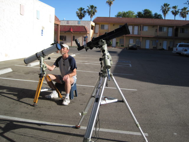
![[Solar annular eclipse of January 15, 2010 in Jinan, Republic of China, by A013231 on Wikimedia Commons.]](http://commons.wikimedia.org/wiki/File:Solar_annular_eclipse_of_January_15,_2010_in_Jinan,Republic_of_China.JPG)
![[eclipse viewed through leaves]](http://commons.wikimedia.org/wiki/File:IMG_1650_zonsverduistering_Malta.JPG)
![[Solar projection with a Dobsonian]](http://commons.wikimedia.org/wiki/File:Home_made_dobsonian_user_to_make_a_solar_projection_%28Split,_Croatia%29_3.jpg)
![[components of the Equation of time]](http://ephemeris.sjaa.net/1201/graph.jpg)
![[analemma in San Jose at noon clock time]](http://shallowsky.com/blog/images/analemma/sj-analemma-clocktimes.jpg) And my 12-noon analemma came out almost vertical! Maybe the tilt I saw
in analemma photos was just a function of taking the photo early in
the morning or late in the afternoon? To find out, I calculated the
analemma for 7:30am and 4:30pm, and sure enough, those were tilted.
And my 12-noon analemma came out almost vertical! Maybe the tilt I saw
in analemma photos was just a function of taking the photo early in
the morning or late in the afternoon? To find out, I calculated the
analemma for 7:30am and 4:30pm, and sure enough, those were tilted.
![[analemma in San Jose at noon clock time]](http://shallowsky.com/blog/images/analemma/sj-analemma-localtime.jpg) Set the observer date to this adjusted time before calculating your
analemma, and you get the much more vertical figure you see here.
This also explains why the morning and evening analemmas weren't
symmetrical in the previous run.
Set the observer date to this adjusted time before calculating your
analemma, and you get the much more vertical figure you see here.
This also explains why the morning and evening analemmas weren't
symmetrical in the previous run.
![[Size of Pluto and Charon vs. the US]](http://shallowsky.com/blog/images/pluto-and-states.jpg)
![[Comet 17/P Holmes]](http://shallowsky.com/images/sketch/cometholmes.jpg)
![[Nautilus with Fibonacci spiral]](/blog/images/NautilusCutawaySpiral.jpg)
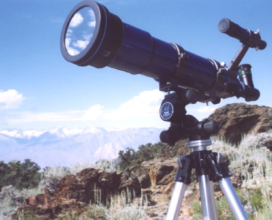